AlbFer

Based on a Siegfried DG9BFC idea, this application shows the temperature of the TRX and the FPGA of ADALM-PLUTO in real-time.

Continue READING

Download SATSAGEN 0.4 and latest versions from this page:

SATSAGEN Download Page

Highlights:

• Dual device mode
• Generator with LO frequency output

Dual device mode

From version 0.4.0, SATSAGEN can handle two devices. In this dual device mode, the first device defined act as RX and the second as TX.

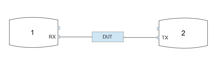
This mode improves the dynamic range of the system because it eliminates the internal crosstalk of devices.

Dual device mode settings

To enable this mode, select Two devices on tab Devices in Settings and specify the device that will act as RX in the first pane and device that will act as TX in the second. If neither devices are specified and the fields Connection string override are left blank, the default URI will be used for devices. The default URI for the first device is ip:192.168.2.1 and the second is ip:192.168.3.1.

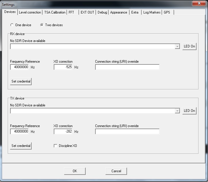
If you have changed the default user and password of devices, you can save these on the program in safe encrypted mode, click buttons, and set credentials. These credentials will be used for sending commands useful to identify the devices uniquely. For example, these credentials will be used by the program to sending the commands to reverse the activity Led blinking of the devices when buttons Led On will be clicked. With buttons labeled Led On you can easily identify a device, the Led activity normal blinking of the related device will reverse.

The settings of the TX device in dual-mode have a checkbox labeled Discipline XO; if checked, the TX device is tuning with periodically XO correction values according to the position and shaping of the signal received in the dual-mode by RX device. These corrections are running during the scans and calibrations only with appropriate RX amplitude. This feature aid in mitigating the drift of the standard TCXO. Without this feature, the drift of standard TCXO in dual device mode can considerably affect the amplitudes read during the scans.

The feature Discipline XO is not active when:

• Frequency is below 71 MHz
• RX or TX offset are specified.
• The TSA scan modality is in multiplier offset or harmonic.
• The RX amplitude drops below -20 dBm for the fine correction according to signal shaping.
• The RX amplitude drops below -60 dBm for the correction according to the signal position.

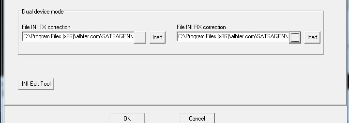
The tab Level correction has a new section in dual device mode where can be specified the custom linearization files for RX and TX devices running in this modality:

Dual device mode operation

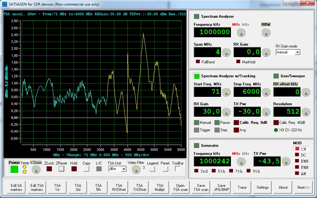
The dual device mode operation is the same as a standard single device; also, the user interfaces not change. The only difference is the small virtual LED in the right lower of the panel of TSA. This LED indicates the Discipline XO feature’s status with green color when normal condition and displays the value used for correction, in this example, -222 Hz.

I suggest before to do a calibration and execute the measures, to let running for some scans with a loopback cable. This trick allows the Discipline XO feature to reach the optimal correction for the TX device.

The best condition is reached when the temperature of devices is in steady-state, mostly when the devices use standard TCXO components.

Generator with LO frequency output

Set the generator to DC to turn off the modulation of the carrier:

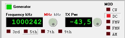
This feature improves the generator output; moreover, the harmonics can be easily calculated because the output frequency is the same as the TX LO. In this mode, a DC is applied to the I and Q input of the TX mixer.

plutotx is a very simple console application that drives Adalm Pluto to generate a CW tone on the frequency and power level selected by the user.

I hope that the information and the C source that you will read below can be a small help for all developers who want to create a new SDR project.

From the archive available for download you will also find the binaries compiled for Windows and Linux x86, so it could also be useful to those who are not developers but simply have an interest in experimenting with Pluto.

Latest Release:

plutotx v.1.1 (04 august 2022)
File size: 705,962  Bytes
MD5 bb0d3b1e42ff892f377fcf5e2cdbb7f3
SHA1 30ade07ad365b23c211f85632c6e9edcb1efdaa0
SHA256 607ae42da31bddaf1528a4dadac7b8ce711a4e2e9ee9210726c3fb2e1d6f673c

- F: 2,147GHz limit
- I: Output bursts issue
- I: Switching off any DDS second tone active
- A: Include, library and instruction to compile under Windows and Linux

Older versions:

plutotx (4 august 2022)
File size: 685,626 Bytes
MD5 e241666bd41a84e5eff1ec44dab2283f
SHA1 e775f8fce1af59c833a850635b6df135cda9ef1b
SHA256 bf1e782b704b5671c901bfb53280a7f754475eba3d0204dd5bf25f99326e393b

To compiling and execute plutotx needs libiio library from ADI. Download and install the library for your specific SO from here: libiio

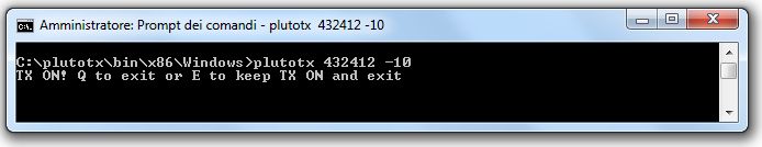
To launch, plutotx requires three parameters: frequency in kHz, a power level output expressed in dBm and a URI of device to connect (optional)

eg.: plutotx 432410 -10

plutotx will connect to default URI of device ip:192.168.2.1 if the third optional parameter is not specified.

How it works

I will describe the source of plutotx in a simplified form to facilitate understanding of the steps required to generate the CW tone:

• Connect to Pluto device and acquire the context structure
• From the acquired context test the model of the transceiver if an AD9364
• Find devices physical transceiver and the DAC/TX output driver (FPGA)
• Find channels of I, Q, TX chain and TX Local Oscillator
• Apply the default configuration
• Set the TX attenuator value
• Set the TX bandwidth
• Set the frequency and phase of the I and Q channels
• Set the frequency of the TX Local Oscillator
• Turn on the TX output activating channels I and Q raw

First of all, we need to connect to Pluto device and acquire the context structure:

struct iio_context *ctx;
ctx = iio_create_context_from_uri("ip:192.168.2.1");

From the acquired context test the model of the transceiver if an AD9364:

if((value=iio_context_get_attr_value(ctx, "ad9361-phy,model"))!=NULL)
  {
  if(strcmp(value,"ad9364"))
    stderrandexit("Pluto not expanded",0,__LINE__);
  }else
   stderrandexit("Error retrieving phy model",0,__LINE__);

Find devices physical transceiver and the DAC/TX output driver (FPGA):

phy = iio_context_find_device(ctx, "ad9361-phy");
dds_core_lpc = iio_context_find_device(ctx, "cf-ad9361-dds-core-lpc");

Find channels of I, Q, TX chain and TX Local Oscillator:

tx0_i = iio_device_find_channel(dds_core_lpc, "altvoltage0", true);
tx0_q = iio_device_find_channel(dds_core_lpc, "altvoltage2", true);
tx_chain=iio_device_find_channel(phy, "voltage0", true);
tx_lo=iio_device_find_channel(phy, "altvoltage1", true);

Apply the default configuration. This step is not necessary probably but recommended if using another SDR application before plutotx:

//enable internal TX local oscillator
if((rc=iio_channel_attr_write_bool(tx_lo,"external",false))<0)
  stderrandexit(NULL,rc,__LINE__);

//disable fastlock feature of TX local oscillator
if((rc=iio_channel_attr_write_bool(tx_lo,"fastlock_store",false))<0)
  stderrandexit(NULL,rc,__LINE__);

//power on TX local oscillator
if((rc=iio_channel_attr_write_bool(tx_lo,"powerdown",false))<0)
  stderrandexit(NULL,rc,__LINE__);

//full duplex mode
if((rc=iio_device_attr_write(phy,"ensm_mode","fdd"))<0)
  stderrandexit(NULL,rc,__LINE__);

//calibration mode to manual
if((rc=iio_device_attr_write(phy,"calib_mode","manual"))<0)
  stderrandexit(NULL,rc,__LINE__);

Line 18 sets the TX calibration mode to manual to avoid spikes on output over the TX power level sets by the user.

Set the TX attenuator value. The attenuator value is calculated from the value requested by the user minus the output power of Pluto that is about 10 dBm defined by REFTXPWR:

if((rc=iio_channel_attr_write_double(tx_chain,"hardwaregain",dBm-REFTXPWR))<0)
  stderrandexit(NULL,rc,__LINE__);

Set the TX bandwidth:

if((rc=iio_channel_attr_write_longlong(tx_chain,"rf_bandwidth",FBANDWIDTH))<0)
  stderrandexit(NULL,rc,__LINE__);

Set the scale, frequency and phase of the I and Q channels:

if((rc=iio_channel_attr_write_double(tx0_i,"scale",1))<0)
  stderrandexit(NULL,rc,__LINE__);

if((rc=iio_channel_attr_write_double(tx0_q,"scale",1))<0)
  stderrandexit(NULL,rc,__LINE__);

if((rc=iio_channel_attr_write_longlong(tx0_i,"frequency",FCW))<0)
  stderrandexit(NULL,rc,__LINE__);

if((rc=iio_channel_attr_write_longlong(tx0_q,"frequency",FCW))<0)
  stderrandexit(NULL,rc,__LINE__);

if((rc=iio_channel_attr_write_longlong(tx0_i,"phase",90000))<0)
  stderrandexit(NULL,rc,__LINE__);

if((rc=iio_channel_attr_write_longlong(tx0_q,"phase",0))<0)
  stderrandexit(NULL,rc,__LINE__);

Set the frequency of the TX Local Oscillator. The TX local oscillator frequency will be the value requested by the user minus the frequency of the CW tone.

if((rc=iio_channel_attr_write_longlong(tx_lo,"frequency",freq-FCW))<0)
  stderrandexit(NULL,rc,__LINE__);

Turn on the TX output activating channels I and Q raw:

int rc;

if((rc=iio_channel_attr_write_bool(
		tx0_i,
		"raw",
		1))<0)
 stderrandexit(NULL,rc,__LINE__);

if((rc=iio_channel_attr_write_bool(
		tx0_q,
		"raw",
		1))<0)
 stderrandexit(NULL,rc,__LINE__);

Entire source code of plutotx:

/*
 Author: Alberto Ferraris IU1KVL - https://www.albfer.com

 This program is free software: you can redistribute it and/or modify
 it under the terms of the version 3 GNU General Public License as
 published by the Free Software Foundation.
 
 This program is distributed in the hope that it will be useful,
 but WITHOUT ANY WARRANTY; without even the implied warranty of
 MERCHANTABILITY or FITNESS FOR A PARTICULAR PURPOSE.  See the
 GNU General Public License for more details.
 
 You should have received a copy of the GNU General Public License
 along with this program.  If not, see <http://www.gnu.org/licenses/>.
 
 */
 
#include <stdio.h>
#include <stdlib.h>
#include <string.h>
#include "iio.h"

#define URIPLUTO "ip:192.168.2.1"
#define MINFREQ 50000000
#define MAXFREQ 6000000000
#define MINDBM -89
#define MAXDBM 10
#define REFTXPWR 10
#define FBANDWIDTH 4000000
#define FSAMPLING 4000000
#define FCW 1000000

struct iio_channel *tx0_i, *tx0_q;

void stderrandexit(const char *msg, int errcode, int line)
{
if(errcode<0)
  fprintf(stderr, "Error:%d, program terminated (line:%d)\n", errcode, line);
  else
  fprintf(stderr, "%s, program terminated (line:%d)\n",msg, line);
exit(-1);
}

void CWOnOff(int onoff)
{
int rc;

if((rc=iio_channel_attr_write_bool(
		tx0_i,
		"raw",
		onoff))<0)
 stderrandexit(NULL,rc,__LINE__);

if((rc=iio_channel_attr_write_bool(
		tx0_q,
		"raw",
		onoff))<0)
 stderrandexit(NULL,rc,__LINE__);
}

int main(int argc, char* argv[])
{
struct iio_context *ctx;
struct iio_device *phy;
struct iio_device *dds_core_lpc;
struct iio_channel *tx_chain;
struct iio_channel *tx_lo;
const char *value;
long long freq;
double dBm;
int rc;
int ch;

if(argc<3)
  {
  printf("Usage: plutotx kHz dBm [uri]\n");
  return  0;
  }

freq=atol(argv[1])*1000;

if(freq<MINFREQ || freq>MAXFREQ)
  stderrandexit("Frequency is not in range",0,__LINE__);

dBm=atof(argv[2]);

if(dBm<MINDBM || dBm>MAXDBM)
  stderrandexit("dBm is not in range",0,__LINE__);

if(argc>3)
  ctx = iio_create_context_from_uri(argv[3]);
  else
  ctx = iio_create_context_from_uri(URIPLUTO);

if(ctx==NULL)
  stderrandexit("Connection failed",0,__LINE__);

if((value=iio_context_get_attr_value(ctx, "ad9361-phy,model"))!=NULL)
  {
  if(strcmp(value,"ad9364"))
    stderrandexit("Pluto is not expanded",0,__LINE__);
  }else
   stderrandexit("Error retrieving phy model",0,__LINE__);

phy = iio_context_find_device(ctx, "ad9361-phy");
dds_core_lpc = iio_context_find_device(ctx, "cf-ad9361-dds-core-lpc");  
tx0_i = iio_device_find_channel(dds_core_lpc, "altvoltage0", true);
tx0_q = iio_device_find_channel(dds_core_lpc, "altvoltage2", true);
tx_chain=iio_device_find_channel(phy, "voltage0", true);
tx_lo=iio_device_find_channel(phy, "altvoltage1", true);

if(!phy || !dds_core_lpc || !tx0_i || !tx0_q || !tx_chain || !tx_lo)
  stderrandexit("Error finding device or channel",0,__LINE__);

//enable internal TX local oscillator
if((rc=iio_channel_attr_write_bool(tx_lo,"external",false))<0)
  stderrandexit(NULL,rc,__LINE__);

//disable fastlock feature of TX local oscillator
if((rc=iio_channel_attr_write_bool(tx_lo,"fastlock_store",false))<0)
  stderrandexit(NULL,rc,__LINE__);

//power on TX local oscillator
if((rc=iio_channel_attr_write_bool(tx_lo,"powerdown",false))<0)
  stderrandexit(NULL,rc,__LINE__);

//full duplex mode
if((rc=iio_device_attr_write(phy,"ensm_mode","fdd"))<0)
  stderrandexit(NULL,rc,__LINE__);

//calibration mode to manual
if((rc=iio_device_attr_write(phy,"calib_mode","manual"))<0)
  stderrandexit(NULL,rc,__LINE__);

CWOnOff(0);  

if((rc=iio_channel_attr_write_double(tx_chain,"hardwaregain",dBm-REFTXPWR))<0)
  stderrandexit(NULL,rc,__LINE__);

if((rc=iio_channel_attr_write_longlong(tx_chain,"rf_bandwidth",FBANDWIDTH))<0)
  stderrandexit(NULL,rc,__LINE__);

if((rc=iio_channel_attr_write_longlong(tx_chain,"sampling_frequency",FSAMPLING))<0)
  stderrandexit(NULL,rc,__LINE__);

if((rc=iio_channel_attr_write_double(tx0_i,"scale",1))<0)
  stderrandexit(NULL,rc,__LINE__);

if((rc=iio_channel_attr_write_double(tx0_q,"scale",1))<0)
  stderrandexit(NULL,rc,__LINE__);

if((rc=iio_channel_attr_write_longlong(tx0_i,"frequency",FCW))<0)
  stderrandexit(NULL,rc,__LINE__);

if((rc=iio_channel_attr_write_longlong(tx0_q,"frequency",FCW))<0)
  stderrandexit(NULL,rc,__LINE__);

if((rc=iio_channel_attr_write_longlong(tx0_i,"phase",90000))<0)
  stderrandexit(NULL,rc,__LINE__);

if((rc=iio_channel_attr_write_longlong(tx0_q,"phase",0))<0)
  stderrandexit(NULL,rc,__LINE__);

if((rc=iio_channel_attr_write_longlong(tx_lo,"frequency",freq-FCW))<0)
  stderrandexit(NULL,rc,__LINE__);

CWOnOff(1);

printf("TX ON! Q to exit or E to keep TX ON and exit\n");

while(1)
     {
     ch=getchar();
     if(ch=='q' || ch=='Q')
       {
       CWOnOff(0);
       break;
       }
     if(ch=='e' || ch=='E')
       break;
     };

iio_context_destroy(ctx);

return 0;
}