
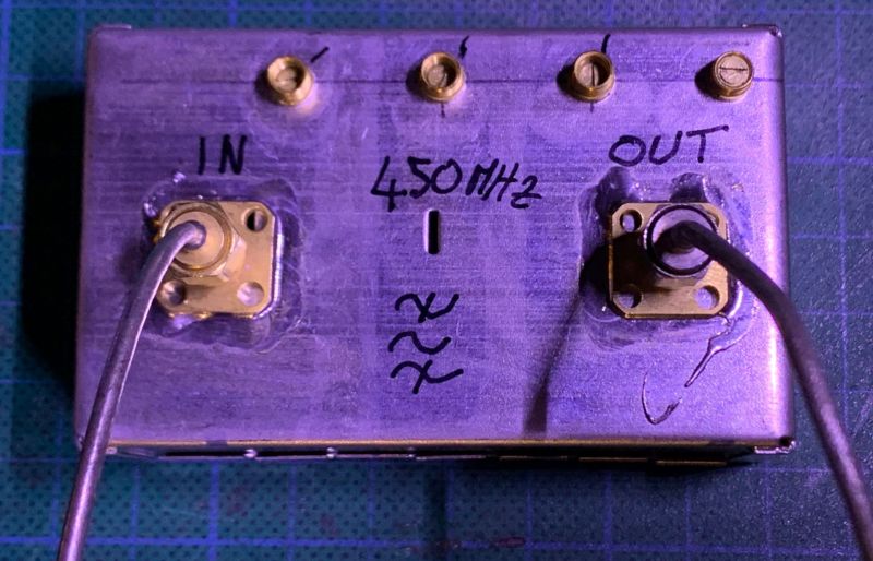
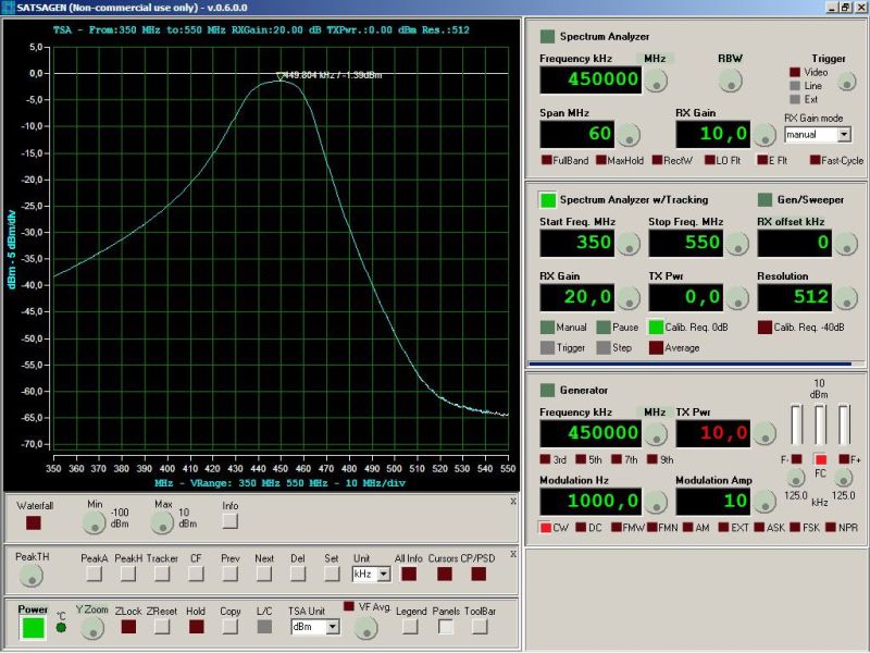
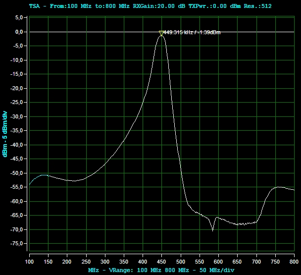
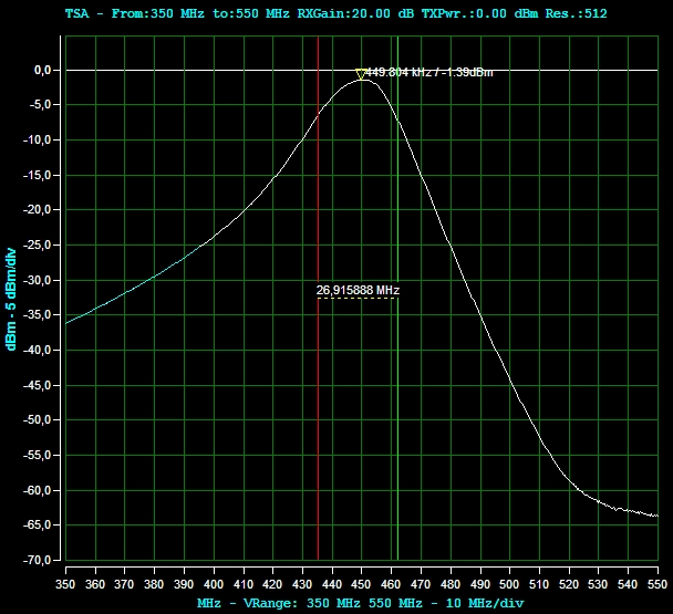
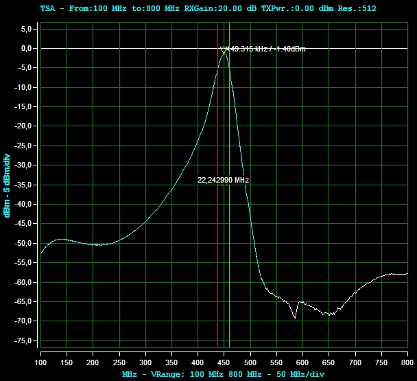
Luigi IZ7PDX made this filter. It is a bandpass centered at 450 MHz that Luigi will use as an IF filter.
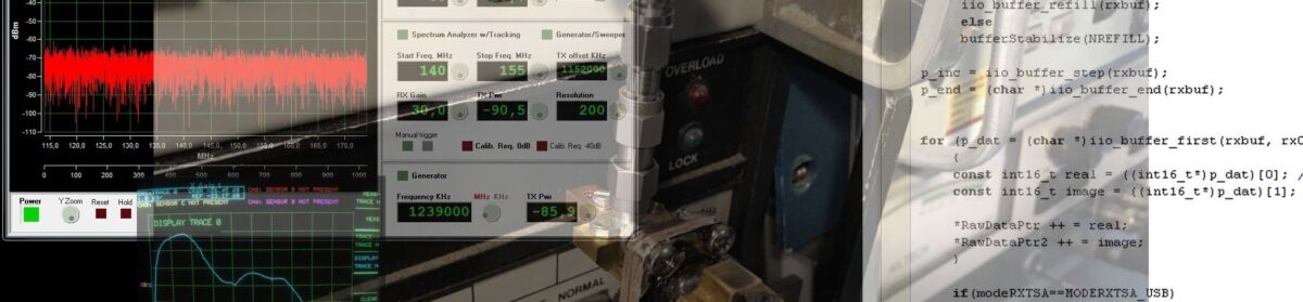
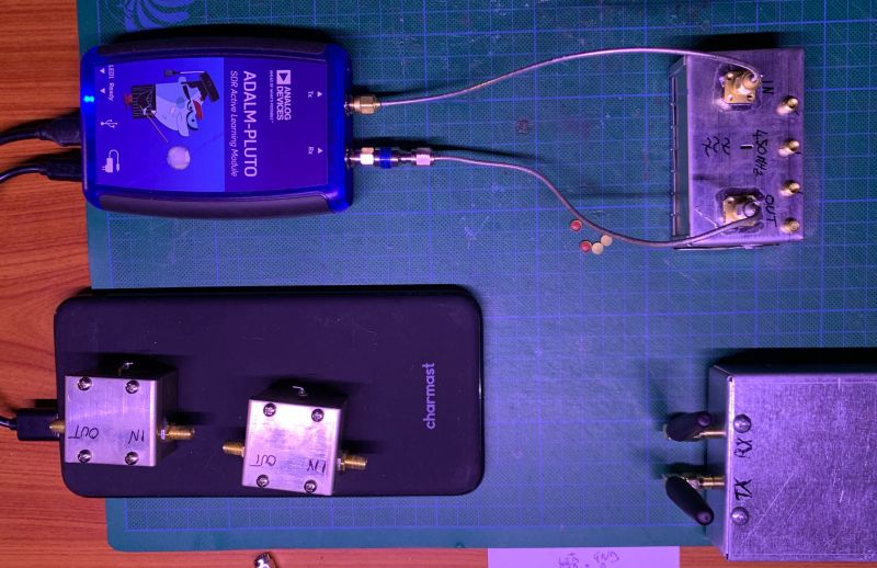
Luigi characterized the filter using ADALM-PLUTO and SATSAGEN.
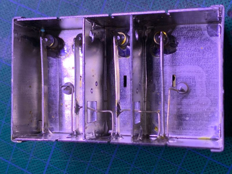
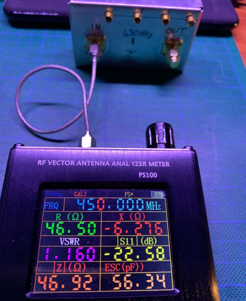
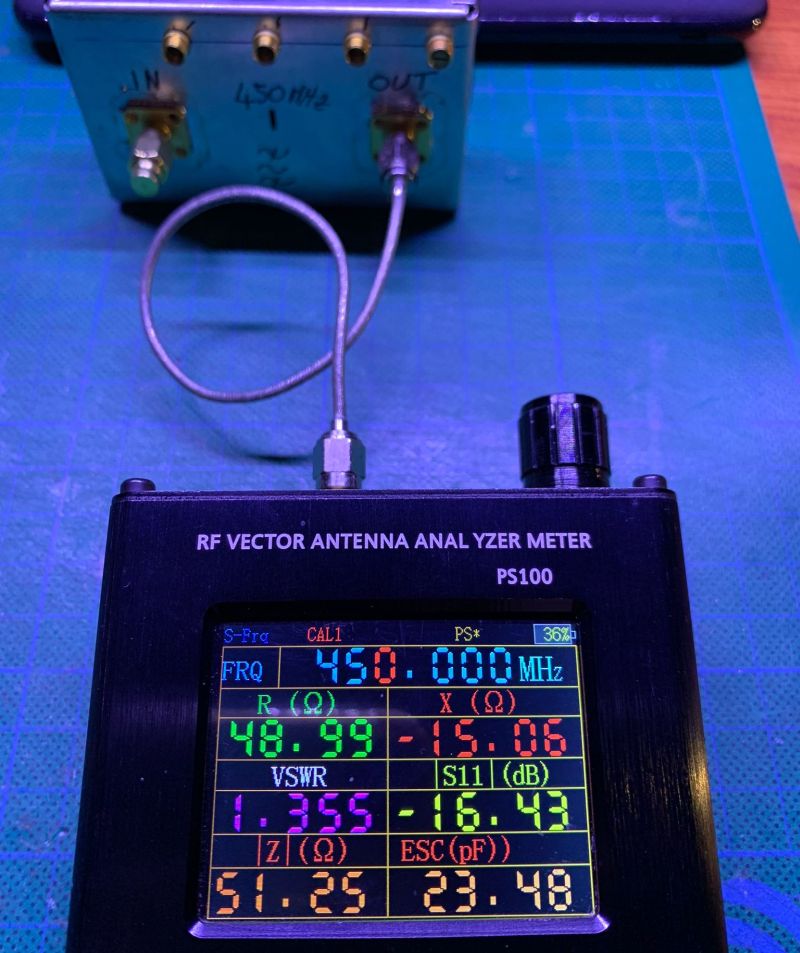
Luigi has further improved the input and output impedance of the filter by acting on the coupling links and measuring with a vector antenna Analyzer:
Find Luigi IZ7PDX on:
- Youtube channel
- Site