Skip to content
AlbFer
Nothing is impossible
Month:
November 2023
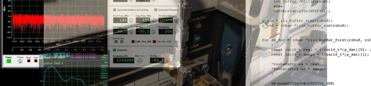
SATSAGEN v.0.8.0.0
SATSAGEN v.0.8.0.0 article
(English Google translated)