

VNA SATSAGEN software with PlutoSDR. Testing by Gianni IW1EPY
First set up from 100 MHz to 6 GHz
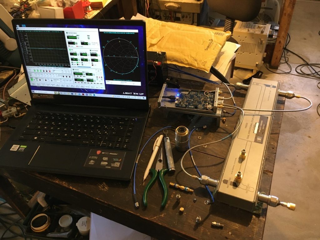
This is the 2 TX 2 RX Pluto (rev C ) using the NEW SATSAGEN SW able to analyze in the complex domain.
The picture shows the setup for the S11 analysis.
A directional coupler is needed, in this case, a dual directional coupler is connected to Pluto.
The TX1 is as usual devoted to the tracking generator and goes to the input of the dir coupler.
The reflected power from the dir coupled goes as usual to the RX1 of Pluto.
The new entry is that the incident power of the dual dir coupler goes to RX2 and is used as a reference.
TX2 is not used in this setup and is switched off.
Another setup can be done using a single dir coupler in this case the TX2 can be used as a reference and connected to RX2.
As with all the VNA, the first step is the calibration phase.
The calibration data of the cal kit can be stored in an appropriate file.
The calibration phase allows measuring 3 different networks (the SOL Cal Kit ) to calculate the correction factor to be applied during the measurement phase.
So at the end of this phase, the setup is calibrated at the plane where the cal kit was applied .. ( end of the N to SMA in this case )
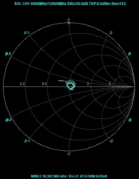
What you can see now…applying the corrections
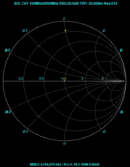
Ending with the Load the calibration and leaving it connected, a dot in the center of the Smith chart will appear or in another format.
Some notes to this image.
The dual directional coupler (HP11692) is certified from 2 to 18 GHz with 30 dB of directivity.
The calibration process allows the use from 0.1 GHz with directivity at last 50 dB and in its range an increase of 30 dB over the HP specs.
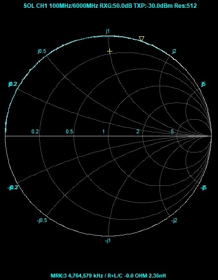
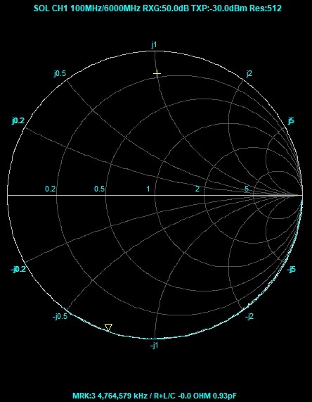
This is what you can see attaching the HP calibration short that, as by specs, is not a short in the reference plane but have an electrical delay (means that there is a line starting at the reference plane followed by the real short).
The line as the frequency increase moves the short on the external circle of the Smith chart.

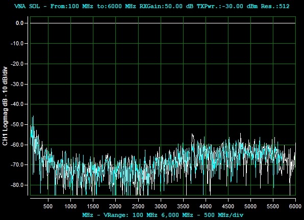
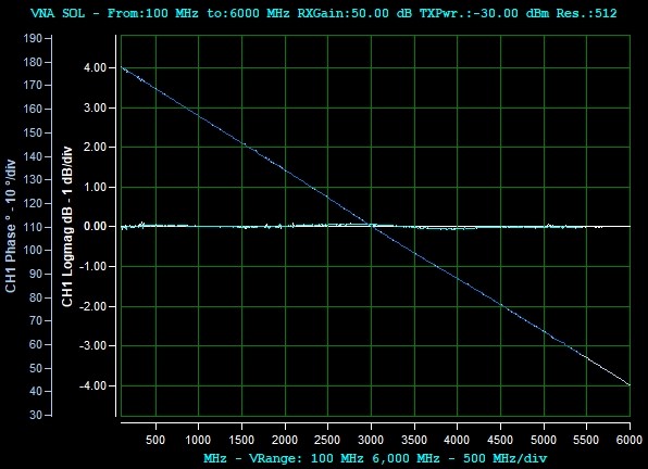
This is another way to see the short behavior 0 return loss ( total reflection ) and a linear increase of phase at frequency increase.
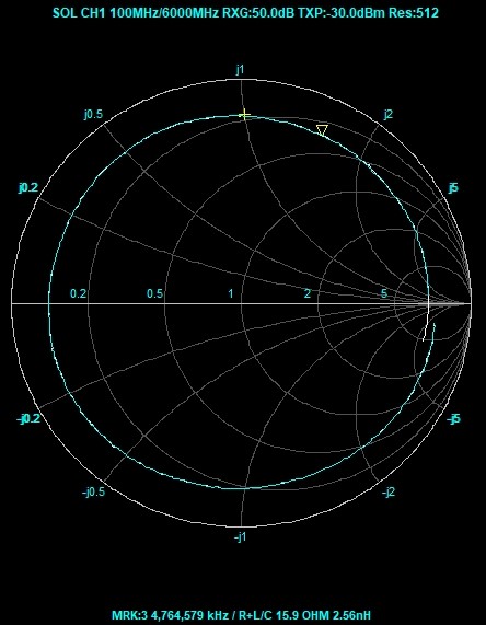
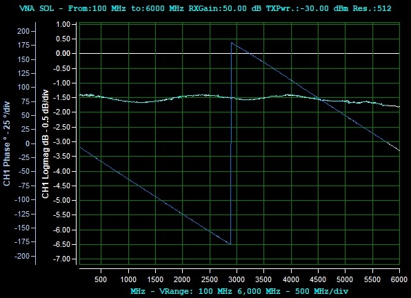
Same for open
The phase roll over every 180 degrees, so similar to the short
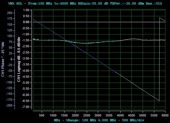
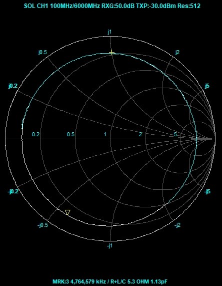
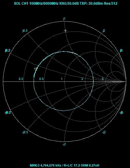
Attaching an attenuator of 1 dB and leaving the other end open, you start from a resistance ( DC ) of 436 Ohm normalized to 50 Ohm, gives 8.72 than the internal line of the attenuator rotates the phase and at the frequency witch the line extends for lambda /4 the transformation return a real impedance normalized to 1.1 equal to 5.5 ohm
Other way to see the attenuator behavior
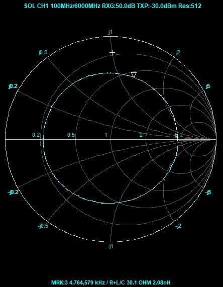
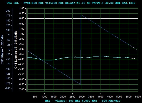
Shorting the other end of the 1 dB attenuator almost the same result
Shorting the other end of the 1 dB attenuator, you reverse the process starting from around 5 Ohm than at lamda/4 to about 450 ohm
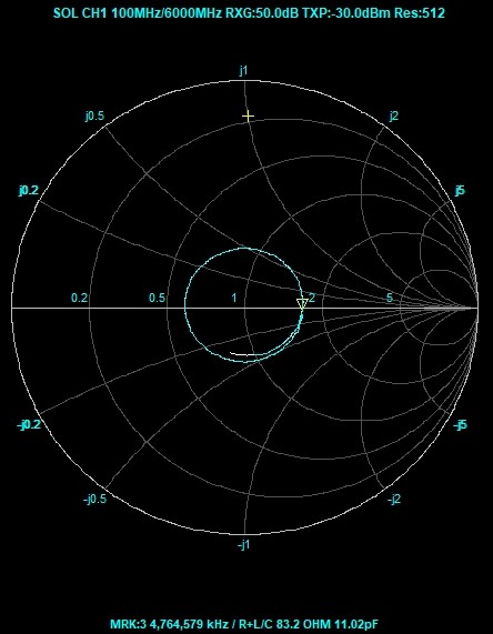
This is the result for a 2 dB attenuator
Is possible to see that the return loss of a 2 dB attenuator on another end open or short gives -4 dB of return loss ( the incident power is reduced by 2 dB in forwarding direction than a total reflection and another 2 dB in the reverse direction for a total of 4 dB of attenuation of the reflected power)
A 3 dB attenuator
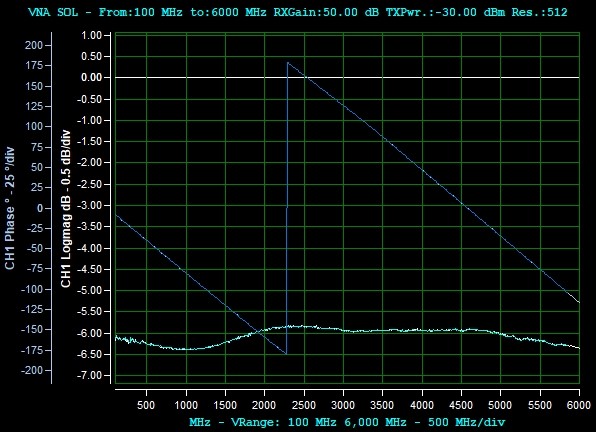
Around -6 dB of return loss for a 3 dB attenuator another end open or short
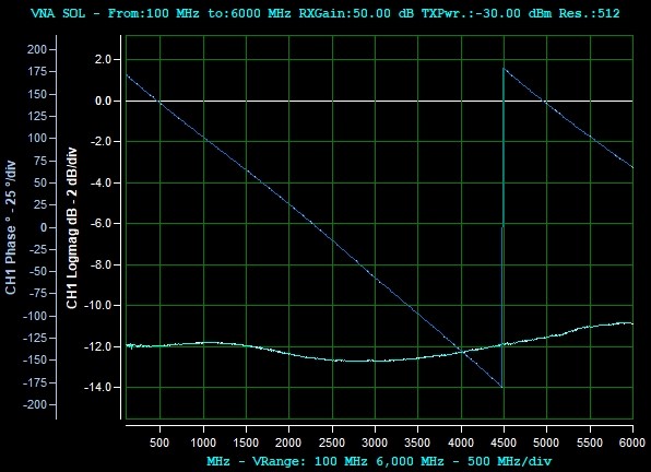
A 6 dB attenuator means -12 dB of return loss.
So inside this circle, every impedance has a return loss better than -12 dB
The same6 dB attenuator
A second 6 dB attenuator is added to the previous 6 dB for a total of 12 dB attenuator, which means -24 dB of return loss.