SATSAGEN v.0.9.0.1

The highlights of this release are:

Radio

The preliminary conditions for using the Radio are:

  • In Settings, Extra tab, if not already active, enable the Multithreading item
  • If you use the Pluto device, check the Kernel buffers item in Settings, Device Options tab
  • The LO F and EF filters in the SA Filters/trace types tab must be turned off
  • The Span must be less than or equal to the maximum instantaneous bandwidth of the device. For example, with Pluto, the Span must be a maximum of 2 MHz (4 MSPS)
  • The resolution bandwidth, in the FFT size entry, must be within a range suitable for the SDR device used. When the Radio is turned on, Satsagen sets the FFT size, if too low, to 4K as a starting point suitable for most devices.

If one or more of the above conditions are not met, the Radio may remain in standby or operate with unsatisfactory listening reproduction.

I decline all responsibility for any damage to hearing resulting from improper use of the audio functions of Satsagen, especially when using headphones.

Before turning on the radio, selecting one of the demodulation modes provided, always set the AF Gain and Volume controls to the lowest possible level, then gradually raise them until the desired reproduction amplitude is obtained.

Bumps, static and other annoying sounds can be reproduced, although it has provided for automatic fading in some occasions, such as when switching from one demodulation to another. These loud and dangerous sounds are reproduced especially using demodulations dependent on the amplitude of the input signal, which is not predictable, such as AM and SSB.

To turn on the Radio:

  • Start the Spectrum Analyzer at the desired center frequency and sufficient RX Gain
  • Activate the Radio tab and choose the desired demodulation from the Mode list:
The radio is active with FM demodulation and 50us of de-emphasis

Once you have chosen the demodulation type, the Radio starts playing on the PC’s default audio.

A tuning cursor, as wide as the selected IF BW, is shown on the display. To move the tuning, click on the display at the position of the desired frequency or by acting on the tuning knob located next to the list of demodulation modes. If the station you want to listen to is outside the displayed span, you must necessarily act on the center frequency of the spectrum analyzer using the usual controls, including those offered by the gesture on the touch screen display.

Double-clicking on the tuning cursor will zoom in to make it easier to center the frequency of the signal you want to demodulate. A subsequent double click in the tuning area will reset the zoom factor to the previous values.

The tuning cursor is a marker visible in the Edit SA markers table as CalcMode DEMOD. When the radio is active, the use of the other markers is not allowed, while it is possible to use the cursors for any measurements.

To turn off the Radio, choose No demod from the Mode list .

The expected demodulations are:

  • AM. The IF bandwidth starts at 12 kHz by default and can be adjusted in the range from 2 to 250 kHz. The AF Gain can reach 45 dB. The tuning can be controlled in 100 Hz steps.
  • N-FM. The IF bandwidth starts at 12 kHz by default and can be adjusted in the range from 2 to 16 kHz. The AF Gain can be set to a maximum of 30 dB. The narrow FM demodulation uses an audio bandpass filter from 200 Hz to 4200 Hz and a 530 uS de-emphasis filter. The use of the squelch is possible. The tuning can be controlled in 100 Hz steps.
  • FM. The IF bandwidth starts from 150 kHz by default and can be adjusted in the range from 2 to 250 kHz. The AF Gain can be set to a maximum of 30 dB. This demodulation does not use any filter other than the AF Filter set by the user. The use of the squelch is possible. The tuning can be controlled in steps of approximately 1 kHz.
  • FM 50uS DE and FM 75uS DE. The IF bandwidth starts at 150 kHz by default and can be adjusted in the range from 2 to 250 kHz. The AF Gain can be set to a maximum of 30 dB. These demodulations are in FM mono. The 19 kHz carrier of stereo broadcasts is partially suppressed by the de-emphasis filter and the AF Filter setting. The de-emphasis filter is 50 uS and 75 uS, respectively. The use of the squelch is possible. The tuning can be controlled in steps of approximately 1 kHz.
  • LSB and USB. The IF bandwidth starts at 2.8 kHz by default and can be adjusted in the range from 2 to 8 kHz. The AF Gain can reach 45 dB. The tuning can be controlled in 1 Hz steps, with the granularity expected by the SDR device in use.

The radio is not compatible with the following Satsagen features: Full Band, Zero Span, NF/G Analyzer, and the LO F and EF filters. If you attempt to use any of the above features at the same time as the radio, the radio will be put into standby, or the features will not activate.

Deviation and modulation amplitude meter

FM deviation and AM modulation measurements can be made with the aid of the Radio.

FM deviation measurement
  • Turn the Radio on to one of the FM demodulation modes
  • The carrier to be measured should preferably be modulated with about 1 kHz and have sufficient power. As a guide, using an ADALM-PLUTO, a carrier of at least -80 dBm is needed. With an RX Gain setting of 40 dB, the measurement tolerance is around 5%.
  • Set a suitable IF BW with the deviation measurement to be performed
  • Center the carrier or tune to the carrier as much as possible
  • Activate the Radio Modulation Metering item from the View menu
  • The third line of text on the tuning slider will display real-time deviation and negative/positive deviation measurements from the center frequency of the tuned channel, in kHz for wide FM and in Hz for narrow FM:
FM deviation measurement, in this example, it is about 79 kHz

To improve the measurement accuracy, perform calibration:

  • Turn the Radio on to one of the FM demodulation modes
  • Tune the carrier, in this case, it must be unmodulated, CW
  • From the Run menu, FM modulation metering calibration item, choose Run Calibration
  • After about a second, if the calibration was successful, measured values ​​around zero should be displayed.
  • Continue with the measurement by now modulating the carrier with approximately one kHz
AM modulation measurement
  • Turn the Radio ON by selecting AM demodulation
  • The carrier to be measured should preferably be modulated with approximately 1 kHz
  • Activate the Radio Modulation Metering item from the View menu
  • The third line of text on the tuning slider will display a real-time measurement of the amplitude in percentage of modulation:
AM modulation measurement, in this example, it turns out to be about 88%

Even in the case of AM, it is possible to perform an a priori calibration to improve the accuracy of the modulation measurement:

  • Turn the Radio on to one of the AM demodulation modes
  • Tune to the desired frequency without the carrier present, so that Satsagen only acquires the noise floor level
  • From the Run menu, AM modulation metering calibration item, select Run Calibration
  • After about a second, if the calibration was successful, you should see fluctuating values ​​below 99%.
  • Continue with the measurement by activating the AM modulated carrier at approximately one kHz

Noise/Gain Analyzer

The Noise/Gain Analyzer functionality has been enhanced to improve measurement accuracy and reduce repetitive calibration tasks.

Adaptive mode

In Settings, Computations tab, enable the new adaptive mode using the Adaptive on three gain settings item :

The Computations tab in Settings, where you enable adaptive mode

The adaptive mode, during the measurement phase, sets the most suitable reception gain for the characteristics of the device under test, thus avoiding false readings following overload of the input stages and ADC of the SDR device used.

Once the adaptive mode has been configured, you can proceed with the calibration and measurement with the same procedure as always, in essence, only the time required for calibration will change, but let’s see in detail what the program does in this new mode:

The calibration phase takes longer to complete than the classic non-adaptive mode, as the program must analyze the behavior of the noise source and SDR receiver system at different Gain levels and then use this information in the measurement phase.

Calibration in adaptive mode consists of the following macro phases:

  • Determine the usable RX Gain range by starting the acquisition with the maximum available RX Gain and progressively reducing it until finding the minimum level where the ON/OFF variations of the noise source can still be used.
  • Divides the above range into three gain levels
  • Perform three calibrations using the three identified gain levels
  • Calculate the maximum measurable gain of the devices under test and map the three calibrations to three DUT gain ranges

During measurement, the program determines which of the three RX Gain levels and associated calibration to use based on the approximate gain of the device under test.

If, during calibration, the program determines that there are no conditions to create three RX Gain ranges, because the deviation between maximum gain and the minimum usable gain is too small, then the adaptive mode is automatically disabled, and the system proceeds classically.

Harmonic compensation

Some SDR devices, such as the Pluto, can introduce a reading error during calibration due to the emphasized harmonic behavior of the receiving mixers and the fact that there is no pre-selector filter at the input. These conditions cause the noise level of the source head to be received not only at the fundamental measurement frequency but also at the harmonic frequencies, more markedly at the third and fifth harmonics. This error is reflected in the measurement results, especially in an underestimation of the Gain of the device under test, in particular, this occurs when measuring narrow-band DUTs.

From this version, Satsagen provides the application of a compensation that significantly reduces the error on both the Gain and the Noise figure measured. To activate this compensation mechanism, simply fill in the Bandwidth field of the marker used for the measurements with the approximate value of the bandwidth of the device under test:

The markers table and the BandWidth column must be filled in to enable the compensation mechanism

The compensation will be calculated by the program based on the characteristics of the SDR used and how it behaves at the harmonic frequencies, combined with the ENR information of the Noise Source table used.

The compensation will be applied only during the final display of the device measurement, that is, when the latter is connected to the system, so it will not be displayed at the end of the calibration, where the Gain and Noise Figure displays will always oscillate around zero.

If you want to know the compensation level already during the calibration phase, activate the Show the mixer’s harmonic compensation at the calibration level item from the Computations->NF/G Analyzer->Session settings menu.

Using TX SDR as Noise Source!

I thought it could be interesting, on an experimental basis, to use the TX part of the SDR as a Noise Source!

Satsagen was already equipped in the generator part with an NPR modulation that allows the measurement of the intermodulation of adjacent channels. In essence, it is a pseudo-random noise generator including three notch filters. The NF/G Analyzer part can be configured to use this generator as a Noise Source for Noise Figure and Gain measurements.

It should be noted that this possibility produces reliable Noise Figure results only if the system is characterized by professional and calibrated instruments, to create a customized ENR table to be inserted into the program. Furthermore, compared to a Noise Source head, the use of an SDR device as a noise source has the following disadvantages:

  • Once the SDR with the attenuator installed has been characterized using calibrated instrumentation, the device must be dedicated only for NF/G measurements; for example, even the simple operation of unscrewing the attenuator and then replacing it can invalidate the characterization just performed.
  • The frequency and power instability of an SDR vs. thermal variations is greater than that of a traditional cartridge and could introduce unacceptable Noise Figure measurement errors.
  • The usable frequency range is usually lower than a traditional Noise Source cartridge. For example, with a Pluto, you can generate noise from about 70 MHz to 6 GHz.
  • Last but not least, an SDR used as a noise source can only be used by Satsagen, while a traditional head can be used with most hardware measurement systems and with Satsagen.

For the above reasons, using a Noise Source head is always the best choice. Since purchasing a branded head is becoming more and more expensive over time, it would be worth trying to build one yourself or choosing emerging products such as those proposed by Mauro IZ1OTT, who offers a portfolio of RF microwave components with an excellent quality/price ratio. Information about this can be found on Mauro’s website: https://www.mauroottaviani.com.

Enabling the TX SDR as a noise source is simple. In SettingsExt In/Out tab, choose the Generator as a Noise Source item from the Noise source power interface list, then in the Computations tab, enter the name of the file containing the ENR characterization table of the TX SDR. I will explain how to characterize an SDR as a Noise Source in the next chapter. For purely indicative purposes, I have inserted some examples of ENR tables of the SDR devices in the Satsagen setup, they can be found in Documents\satsagen\settings\ENRTables. The names of the example files are composed in this way: an ENR prefix followed by the name of the SDR device and optionally the sampling frequency used in the characterization. The file name always ends with a suffix indicating the value of the TX attenuator used. For example, the name of the table for the ADALM-PLUTO at 8 MSPS with a 20 dB attenuator is: ENRADALMPLUTO8MSPS-20. If the sampling rate is not specified in the name, the table is suitable for the worst case condition of using the SDR TX as Noise Source, where the device is used simultaneously also as RX and the baseband is shared, so the sampling rate is fixed by the receiving side and may not be the optimal one, as in the case of ADALM-PLUTO at 8 MSPS.

The SDR devices considered by Satsagen as Noise Source are:

  • ADALM-PLUTO and accessories with 20 dB attenuator on TX connector
  • USRP with 30dB TX attenuator
  • AntSDR E200 with 30dB TX Attenuator
  • HackRF One with 50 dB TX attenuator
Characterization of an SDR TX as a Noise Source

For ENR characterization of a device, a reliable and calibrated ENR measuring instrument is required.

Below is the procedure to characterize an ADALM-PLUTO as a Noise Source:

The setup must match the final measurement setup, so for example if you will use the NF/G Analyzer with a single ADALM-PLUTO device with the roles of both receiver and Noise Source (the worst condition in terms of measurement reliability), the characterization setup will be a single ADALM-PLUTO with a -20 dB attenuator on the TX connector. If you have two ADALM-PLUTOs available, one to dedicate to reception and another as a Noise Source, then the characterization setup could be composed of two ADALM-PLUTOs, with the device dedicated to the Noise Source equipped with a -20 dB attenuator on the TX connector.

  • Connect the TX (obviously the attenuator output) to the ENR measuring instrument
  • In SettingsExt In/Out tab, choose the Generator as a Noise Source item from the Noise source power interface list
  • Create as many markers of type CalcMode NF/G with a span of 400000 at the frequencies you want to characterize in increasing order. For example, 71000000, 100000000, 144000000, 432000000, and so on.
  • Select the first marker with the lowest frequency
  • Start the NF/G Analyzer by clicking the ON button in the NF/G Analyzer tab.
  • Configure the ENR measurement tool with a bandwidth corresponding to half of the value displayed in the Sampling kHz box of the Satsagen generator.
  • Click the small TX On button on the generator and note the frequency and ENR value read on the meter
  • Select the next marker and click the TX On button again, and note the frequency and ENR value displayed by the meter. Repeat this step for all created markers.
  • Open in Settings, tab Computations, the ENR file writing tool via the ENR INI Edit Tool button, and copy the frequencies and ENRs noted in the table. Then save via the Export button to an ENRADALMPLUTO-20.ini file
Saving calibration data

The NF/G Analyzer system from this version will automatically save the calibration data. The saved data can be reused to perform new measurements, saving the time needed for calibration. For example, it is now possible to perform a calibration and measurement of a DUT, close the application, reopen it, and perform the measurement on a new DUT with the same frequency and bandwidth characteristics, skipping the calibration phase. It is also possible to calibrate the system on multiple frequencies and bandwidths and subsequently perform the measurement on multiple DUTs, without having to recalibrate the system each time.

Using this new feature is very simple. If there is calibration data in memory, usable for the characteristics of the currently selected marker, then a small LED next to the calibration button will turn yellow:

The small yellow LED next to the SYS CAL button

At this point, you can decide whether to use the data in memory or perform a new calibration and measurement cycle. To use the calibration data in memory and immediately start measuring the DUT, click on the SYS CAL button while simultaneously holding down the CTRL key on the keyboard. The SYS CAL button will immediately turn green to indicate the correct recovery of the calibration data and the start of the measurement phase. Instead, to ignore the presence of saved calibration data and perform a new calibration cycle, thus overwriting the data in memory, simply click on the SYS CAL button as usual.

For the system to propose calibration data as reusable, some configuration parameters of the new measurement must be identical to those saved, the main ones being:

  • Same type of measurement: Manual, Auto, or Auto Adaptive
  • Same Frequency
  • Same IF Frequency if specified
  • Same Bandwidth (Span)

If one or more of the above main parameters do not match, then the small LED dedicated to signaling the presence of reusable calibration data will remain off.

To view the list of calibration data stored in memory, select the List the saved calibration data to the trace log item from the Computation->NF/G Analyzer->Calibration data menu :

An example of a list of saved calibration data

If there are reusable calibration data that match the above main parameters, but one or more secondary parameters that could affect the accuracy of the measurements differ, then the small LED will turn red, and it is possible to use the information displayed in the balloon tip to trace the non-corresponding parameters:

The small LED next to the SYS CAL button is red due to parameter 24 not being consistent with the saved calibration data

In this example, the current configuration parameter that does not match the saved one is #24. To find a description of the parameter starting from this number, choose the item Dump the selected calibration data to the trace log from the Computation->NF/G Analyzer->Calibration data menu :

An excerpt of the saved calibration data of the currently selected NF/G marker

In the example, the parameter that differs is related to the temperature of the working environment, which is 296 Kelvins in the saved data, while, for example, it was changed by the user in configuration to 290 Kelvins.

ENR Meter

The Satsagen NF/G Analyzer can be used to measure the ENR of a noise source. It should be noted that to perform this measurement, a perfectly characterized Noise Source head needs to be used as a sample. Furthermore, this meter cannot replace professional and calibrated equipment, as the errors introduced by the SDR system can accumulate and lead to unsatisfactory results. In this regard, it is recommended for these measurements to use an SDR that does not have mixers with emphasized harmonic behavior, such as an RTL-SDR, with which it is possible to measure ENR with good results up to about 1.4 GHz.

  • Set up the system as if you were going to make traditional Noise Figure and Gain measurements. If necessary, see this post where I illustrate the basics for using the NF/G Analyzer.
  • Disable the Adaptive on three gain settings item from Settings, Computations tab, as this mode is not compatible with ENR measurement
  • Activate the ENR measurement item from the Computation->NF/G Analyzer->Modes menu
  • Create as many markers of type CalcMode NF/G with a span of 400000 at the frequencies you want to characterize in increasing order. For example, 71000000, 100000000, 144000000, 432000000, and so on.
  • Connect the Noise Source sample head
  • Select the first created marker
  • Start the NF/G Analyzer by clicking the ON button in the NF/G Analyzer tab.
  • Click on SYS CAL and wait for the acquisition to finish when the button turns green
  • Select the next marker and repeat the procedure by clicking on SYS CAL, then continue for all the remaining markers. In this way, the system will store the ENR data of the sample head
  • Connect the Noise Source head to be characterized
  • Select the first marker
  • While holding down the CTRL key, click on the SYS CAL button
  • Note the ENR reading:
The central display shows the ENR dB value
  • Select the next marker and hold down the CTRL key, click on SYS CAL. Then continue with the remaining markers.
Miscellaneous, new configuration parameters

In Settings, Computations tab, you can specify these new parameters to refine the accuracy of the NF/G Analyzer measurements:

The new configuration parameters for the NF/G Analyzer

NS ON/OFF is a delay time that the system introduces after turning the Noise Source head on or off before continuing reading. It can be specified in milliseconds or in drop samples; click on the unit title to switch from one to the other.

Ambient temperature can be specified in degrees Celsius or Kelvin

The Loss 1 and Loss 2 fields allow you to specify the insertion loss of cables or connectors used to connect to the input and output of the DUTs, which are not covered by the calibration.

Average/Time and Cumulative Folding

Average/Time and Cumulative are folding methods that allow discrimination signals from background noise, especially used in radio astronomy.

Average/Time Folding

It is a filter that is selected from those available in the VFilter Type list, with the Folding item :

The VF F knob for controlling the Folding parameters currently selected for AVG cycles

This filter works only with active Multithreading and with Span values ​​lower than or equal to the maximum instantaneous bandwidth of the device, so, for example, in the case of an RTL-SDR, it is equivalent to 1 MHz, or for an ADALM-PLUTO rev B, it corresponds to 30 MHz. If one or more of the above conditions are not satisfied, then the filter will deactivate, and the VFilter Type message will flash red.

Description of operation: The data displayed on the spectrum are first processed by a classic average filter that averages them over several steps that the user can specify from 1 (disabled) to 30 using the VF F AVG knob. In the above example, the average filter is configured for 17 cycles. The data are then inserted into a shift register composed of many blocks that the user can specify with the same knob positioned on VF F Blocks :

The currently selected Folding parameter control VF F knob changes the number of shift register blocks.

In the example, the filter shift register consists of 2362 blocks.

The data is then processed by the shift register and displayed. In the example, the shift register output will be the average of the last 2362 blocks over a period (Folding Period) determined by the size of the pre-filter average and the number of blocks in the register, which period is estimated in real time and displayed in seconds next to the knob, 32 seconds in our example.

Since the memory consumption of this filter can reach high values ​​due to the amount of data present in the shift register corresponding to the spectrum data in the resolution determined by the FFT size multiplied by the number of blocks constituting the register, the system limits its size to approximately 1 GB of RAM maximum.

Cumulative Folding

Cumulative Folding is implemented in Satsagen starting from the raw data processed by the FFT in a separate flow, therefore independent from the VFilter filters and from what will be displayed on the main spectrum display. The Cumulative Folding results are displayed in an independent window in a dedicated display, where the amplitude is expressed in mW.

Cumulative Folding is started with the SA cumulative folding entry from the Run menu.

In essence, Cumulative Folding folds the spectrum back on itself by simply adding it algebraically, repeatedly, until the user stops it using the same Run -> SA cumulative folding menu item or when one of the following events occurs:

  • Complete closure of the Satsagen program
  • Changing the center frequency, span or resolution bandwidth of the Satsagen spectrum analyzer

While the action of turning the spectrum analyzer off and on again only implies a momentary interruption of the Cumulative Folding.

The exposure time accumulated by Folding is displayed in seconds in the title of the dedicated window display.

The same title displays the name of the backup file where the program automatically saves the results every 10 seconds or so.

The files are saved in the documents\satsagen\export folder and can also be opened offline for viewing via the File menu and the Load Cumulative Folding Data item. From this view, it is also possible to export the data in CSV format via the File menu and the Save as CSV item.

If you accidentally restart Cumulative Folding, you can still restore the acquisition with the accumulated and saved data using the following procedure:

  • Start a new acquisition
  • From the File menu, choose Load cumulative folding data and open the interrupted recording file from the documents\satsagen\export directory.
  • From the File menu of the same upload window, select the Merge item and confirm your wish to merge the data from the file just uploaded into the current acquisition session.

Improvements and additions

Configuration profiles

From this version, in addition to the main shortcut icon, the setup creates three additional shortcuts to the Satsagen program with three distinct configuration profiles: SATSAGEN Config #1, #2, and #3.

The four shortcuts created by the Satsagen Setup

The three additional configurations are completely separate, it is possible in this way to start a total of four instances of Satsagen (not necessarily at the same time) with four distinct configurations, to be possibly dedicated to the use of the NF/G Analyzer, or the VNA, or the power meter and so on, without necessarily having to modify the configuration to adapt it to the devices and functions that are needed from time to time.

The title of the SATSAGEN main window displays the number of the configuration currently in use.
Filter Smoothing in seconds per dB

A Smoothing filter type has been added, selectable from the VFilter Type list as Smooth S/dB.

In the traditional Smoothing filter, the display of the received signals is “smoothed” by adding a fraction of dBm set by the user at each pass, until the real power is reached.

In this filter, the full power display of signals is achieved in terms of seconds per dB that can be set by the user, from a minimum of 0.01 seconds per dB to a maximum of 600 seconds per dB.

Assuming a CW signal at -90 dBm, a noise floor of about -100 dBm, and a Smooth S/dB setting of 1 second/dB, the above signal will appear to grow progressively to -90 dBm in about 10 seconds.

In this way it is possible to discriminate signals that have a defined continuity over time.

DC Bias on RX Connector

Some SDR devices (such as the RTL-SDR, AirSpy, HackRF and others) can provide a DC voltage on the RX connector useful for possibly powering external antenna amplifiers.

By default, this option, if present on the device, is disabled.

From this version of Satsagen, it is possible to manually enable the DC Bias by going to the Settings->Device session settings menu and selecting Enable DC Bias Antenna.

If the receiving device does not provide this option, the menu item will be disabled.

Since the DC voltage supplied by the SDR can damage any sensitive devices such as attenuators or other directly connected SDRs that have a DC coupling, the enabling will only be valid within the connection session to the device, so when the program is restarted, or at a Power Off/On cycle, the DC Bias will be disabled and will have to be manually turned on again if necessary via the aforementioned menu item.

Additional safety is provided by the confirmation message for enabling DC bias that will be displayed after selecting the Enable DC Bias Antenna item:

The confirmation message for enabling DC Bias
Generator, TX On button

In the Generator panel, I added a TX On button that can be used to turn the TX output off or on.

The small TX On button on the Generator panel

Compared to the button that starts the Generator, the TX On has an immediate response because it acts directly on the output stages, while the Generator start button determines and prepares the configuration of the SDR device based on the user settings and then starts the output stream, so, for example, the creation in memory of a 10 Hz modulation stream can require a waiting time that can even exceed a second, depending on the characteristics of the PC in use.

If Satsagen is configured in dual-device mode, where one device has an exclusive role of RX and the other of TX, it is possible to enable the Discipline XO item in the Device Options of the TX device box. This feature has been present for some time in the history of Satsagen versions and is a mechanism that automatically adjusts the correction on the reference clock of the TX device to keep it constantly aligned to the RX frequency during Spectrum Analyzer scans with tracking.

Since I have found that it can be impractical to enable or disable this XO discipline feature from Settings when necessary and thus block the scan in progress, I have added a context menu that allows this maneuver (and more) during scans by simply right-clicking in the status area of ​​the Spectrum Analyzer with tracking panel and choosing the desired action:

The pop-up menu that allows you to control the XO disciplines function during scans
Multithread Max instant bandwidth

With multithreading enabled, Satsagen runs a series of dedicated processes that take care of acquiring the data stream from the SDR device in real time.

This only happens if the Span set by the user falls within the maximum instantaneous bandwidth of the SDR device.

If the PC/USB or Ethernet/SDR system is not fast enough, overflows occur, which are counted and displayed under the spectrum display as OF.

In extreme situations, where the frequency of overflows is high, certain SDR devices may experience hangs or the acquisition threads may terminate unexpectedly, stopping the spectrum display.

To avoid the aforementioned crashes and unexpected closures, it is possible to set in the configuration the maximum instant bandwidth beyond which Satsagen turns off real-time acquisition by switching to a slower mode, which, however, no longer produces crashes and unexpected closures.

To set this threshold, go to Settings on the Extra tab:

The selector to set the maximum instant bandwidth

The Max instant bandwidth entry is set by default to the maximum speed of the device (Device MAX); it is therefore possible to position it from a minimum of 5 MSPS up to a maximum of 56 MSPS. The correct value must be found by carrying out tests, for example, starting from the lowest value and increasing it until the system “holds” without causing unexpected blocks or closures.

SATSAGEN INTERFACE

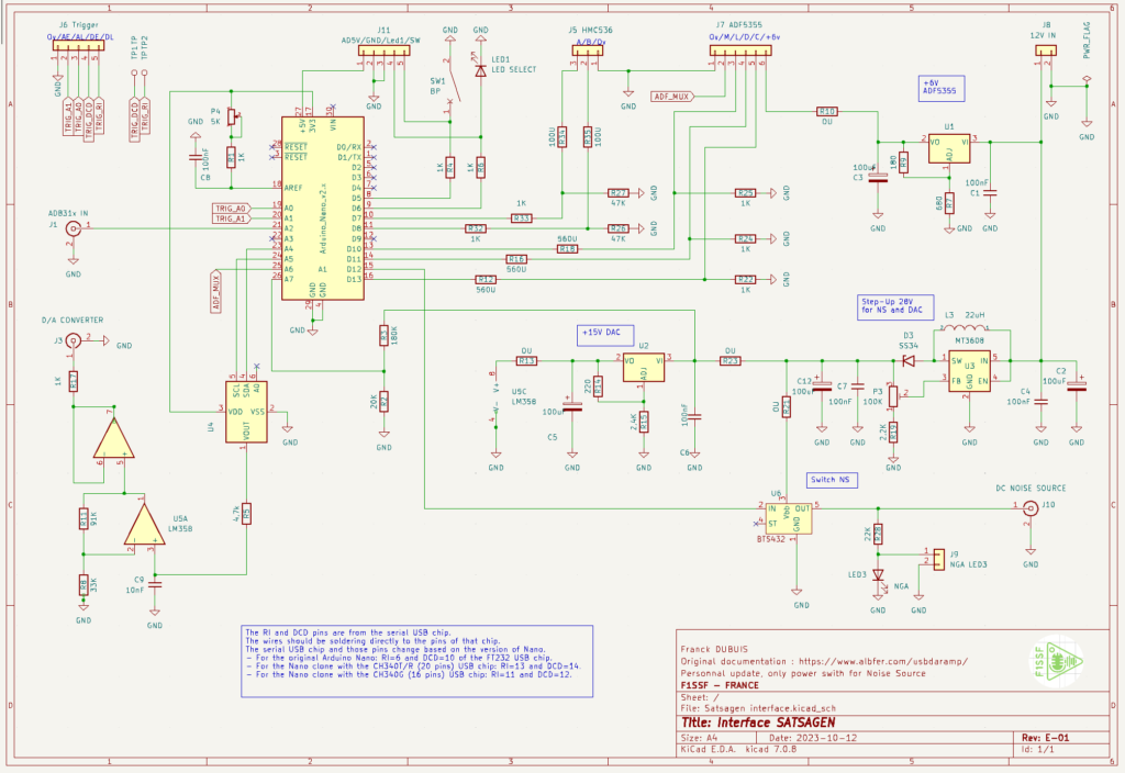
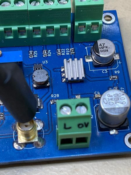
Franck F1SSF has produced an interesting PCB that collects all functions and schematics of the USBDAALBFER interface project (Video).

Franck's SATSAGEN INTERFACE REV. E
Franck’s SATSAGEN INTERFACE REV. E


With SATSAGEN and Franck’s PCB, you can:


Download the Gerber files here or contact Franck F1SSF, but his PCB availability is limited.

Download the Arduino sketch here to compile and upload it to the interface.


Follow Franck’s instruction steps to wire and make operational his SATSAGEN INTERFACE PCB:

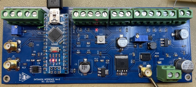
Hi All, Some information here. This PCBA is the first realization:

  • Inserted components except Nano and resistors 0U:
    • Use IBom:
  • Power UP:
    • Power supply on 12V IN connector
  • ADF5355 power supply
    • Measure R10 pad = 6V, if OK solder R10=0U
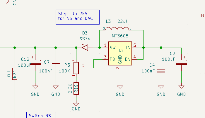
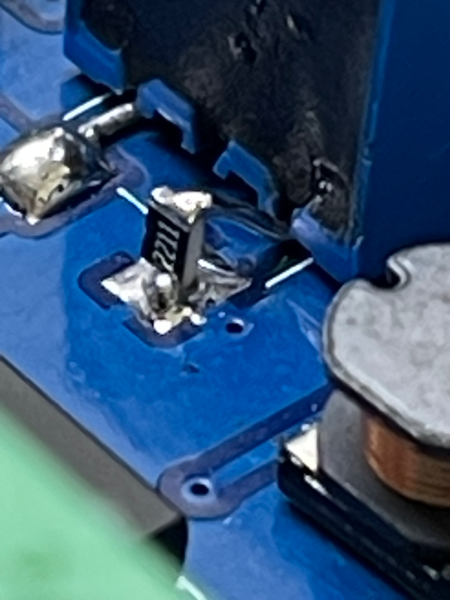
  • Step Up 28V – Warning, add modify R19 as below picture
    • Measure R23 pad, adjust P3 to obtain 28V max, If OK solder R23=0
  • Detector Step Up = ON:
    • Measure divider R2/R3, you must have 3Vmax
  • +15V DAC
    • Measure R13 pad = 15V, if OK solder R13=0U
  • Power OFF
  • Solder wires directly on serial chip Arduino (see schematic for pin numbers)
    • Plug Arduino on support for removal easily, and solder wires DCD = TP1, RI=TP2
  • Check the values of the ADF5355 voltage dividers
    • R12/R22. R16/R24. R18/R25
  • Now you can connect all peripherals
    • Use connectors J6 , J11, J5, J7, J10
  • +3V ref
    • Adjust P4 to have +3V on Arduino pin ref N°18
  • Configure Satsagen in tracking mode 0 to 6Ghz
    • See on J3 voltage ramp from 0V to about 12V.

SW1 allows you to select the operating modes of the Arduino, depending on the use.

You can deport SW1, LED1, and LED3 on the front end with J11 and J9.

If you move the LEDs, then remove the SMD LEDs or if you leave them, then change the R6 and R22 to adapt the current. SW1 can stay on board.

J1 / J2 / J10 Footprints are BNC connectors, but you can use SMA connectors after cutting legs. You solder ground around directly around the body.

Because the ADF5355 consumes approximately 200mA, it is recommended not to exceed 12V power supply to reduce the dissipation of the 6V regulator. I added a small radiator with thermal glue.

If your RF switch HMC536 already contains 100U resistors on ports A and B under the shield, replace R34 and R35 with 0U.

73’s  Franck F1SSF

Franck’s Satsagen Interface schematic Rev E-01

MT3608 step-up 28 Volts section schematic with the R19 to add

The 2k2 R19 to add

The 6 V regulator with a small radiator

SATSAGEN v.0.8.0.0

Highlights

Important changes in Satsagen 0.8.0.0

I leave the list of important changes to read at the end of the article to avoid any difficulties using this new version. Maybe they should have been placed here, but I hated to take up too much space at the top of the main points!

Noise Figure and Gain Analyzer

The NF/G analyzer integrates into the Satsagen spectrum analyzer, which is based on the Y-factor method. Markers help configure the frequencies, IF, and bandwidth of the devices under test.

You will need:

A noise source with an attached ENR characterization table and an SDR device with adequate sensitivity are needed to perform the Noise Figure and Gain measurements. Furthermore, an interface capable of supplying the noise source with 28V and that can be controlled by the application would be necessary, but optional.

I have obtained reliable and comparable results with instruments such as the Eaton 2075 using an ADALM-PLUTO or an RTL-SDR v3 as SDR receivers. The maximum usable and recommended bandwidth for measurements is about 1 MHz with ADALM-PLUTO and 500 kHz with RTL-SDR v3. However, higher bandwidths can be used with the aforementioned two SDR devices at the expense of measurement times and precision.

The noise source I used in testing is an NH 5-12 built by Mauro IZ1OTT and characterized in comparison with an HP 346B. Mauro’s NH 5-12 has an average ENR of about 6.67 dB from 40 MHz to 10368 MHz.

Other Satsagen supported SDRs can be used in addition to those listed above, but from what I have been able to ascertain, there is no guarantee of success in the measurements for all the standard amateur radio frequencies covered by SDR devices without the use of additional LNAs placed before the SDR input to improve their sensitivity.

The quality of the measurements is linked to the noise source and SDR binomial. About the noise sources, it is important to have an ENR value that is sufficient, but not excessive, and characterized in a table using professional instrumentation. For SDRs, reception sensitivity and an adequate SNR are important.

Some notes on this from Mauro IZ1OTT:

<<Given the low sensitivity of SDRs, it is recommended to place a preamplifier between the DUT and the SDR, especially when measuring DUTs with low Gain (< 20 dB) or even zero. Regarding the ENR of the sources, only commercial heads already have a table with values ​​around 15 dB, therefore suitable for any type of measurement. Lower ENRs, obtainable by interposing an attenuator, can improve the measurement precision for low NF (ENR~NF), due to a better adaptation between DUT and source.>>.

Follow a first empirical test to exclude that your SDR/noise source system is completely unusable:

– Make a calibration

– Keeping the noise source connected directly to the SDR RX

– Check the read noise figure and gain values ​​do not oscillate beyond +/- 0.2dB for all the measurement frequencies that interest us.

As for the power supply interface of the noise source – at the time of writing this article – there are two choices supported by Satsagen: use an Arduino Nano or compatible with this sketch and a Step-Up converter plus an optocoupler ( simplified circuit diagram, circuit diagram with voltage control) or use the RTS line (active high) of the serial port of your PC (or a USB/Serial interface) that drives an optocoupler or a mosfet connected to the 28V power supply. It must be said that Satsagen still offers the possibility of one-shot measurements even without the above interfaces; in this case, it is necessary to power the noise source manually in the calibration and measurement phases, all at the expense of convenience and speed in the measurements.

Finally, to improve the impedance matching towards the SDR input, I recommend inserting the usual 1 dB (or at most, 3 dB) attenuator at the SDR RX input.

Preliminary operations :

ENR Table Insertion

First, the ENR table must be inserted into the Satsagen configuration to load it at each program startup. Run Satsagen, go to the Settings->Computations tab, open the ENR table editing tool by clicking on the ENR INI Edit Tool button:

Now enter the ENR values ​​of the noise source at our disposal (remember to select the Append box to make data entry easier), as follows, for the source noise I used:

Once the compilation is complete, export by clicking on the Export button to a file, for example Documents\satsagen\settings\mioENR.ini. Close the tool and enter the above complete path in the ENR INI File box and click OK (to make the entry easier, click on the … button to directly select the file):

SDR selection and power noise source pilot interface

Proceed as follows using an ADALM-PLUTO as SDR:

Go to Settings->Devices and choose, as usual, the SDR device you will use, in the example, an ADALM-PLUTO. Keep the other settings as shown in the images:

Then go to the EXT in/Out tab and configure the interface by selecting Noise source power interface from the list:

Measuring a DUT amplifier:

For example, we have a 23cm bandwidth LNA whose noise figure and gain we want to measure in a bandwidth of 400 kHz:

  • Start the SATSAGEN spectrum analyzer
  • Open the marker table by clicking on the Edit SA markers button on the toolbar
  • Fill in the ReqFrequency fields with the desired frequency in Hz, in this case 1296000000, Span (this is the bandwidth) with 400000, and CalcMode with NF/G (choose the NF/G item from the drop-down menu). We confirm the creation of the marker by clicking on the Post button in the toolbar:
  • At this point, click on the ON button of the NF/G Analyzer tab:
If you notice unwanted components or other transients in the spectrum within the gray acquisition window, you can move that window (the marker) using the J and K keys on your keyboard or the mouse wheel, until the window includes a “clean” spectrum with only the noise floor, trying to avoid including the DC component present in the center.

SATSAGEN will automatically configure all spectrum analyzer parameters such as center frequency, Span, RX gain, FFT size, video filter size, and more, compliant with DUT gain and noise figure measurement. It should be noted that, once the measurements are completed, SATSAGEN will reset all modified spectrum analyzer parameters to the previous user values.

  • Connect the noise source to the Pluto RX port and start the system calibration by clicking the Cal SYS button on the NF/G Analyzer panel. After about 12 seconds, the calibration should complete, and the Cal SYS button should turn green.
The noise source power interface in this image is more complex than necessary; it is a prototype with other functions, including digital and analog trigger inputs, the ability to drive PLL synthesizers such as the ADF5355, and RF switches for use in VNA mode.
System calibration is complete.
  • Connect the DUT and power it, and after a few seconds, we will get the relative noise figure and gain measurements.
SATSAGEN reports a DUT gain of approximately 14.5 dB and a noise figure of 4.0 dB at 1296 MHz.

The DUT amplifier measurements are finished. Close the NF/G analyzer by clicking the green ON button on the NF/G Analyzer panel or by turning off the Spectrum Analyzer.

Measuring a converting DUT, such as a transverter:

To measure a converting DUT, proceed in the same way as previously seen for the amplifier DUT, with the only difference in filling in the marker, where for converting DUTs, you must also enter the IF frequency, or the local oscillator of the device under test. If you measure as a down-converter, the IF frequency must be entered with a negative sign.

For example, we have a 13cm transverter and we want to measure it as a down-converter from 2304 MHz to 144 MHz:

  • Start the SATSAGEN spectrum analyzer
  • Open the marker table by clicking on the Edit SA markers button on the toolbar
  • Reuse an old record of type CalcMode NF/G, or create a new one, fill in the fields ReqFrequency with 2304000000, Span with 400000, IF Frequency with -2160000000, and CalcMode with NF/G. Confirm the creation/modification of the marker by clicking on the Post button in the toolbar.
  • Click the ON button on the NF/G Analyzer tab to start the analyzer:
As you can see, the spectrum analyzer tunes to the transverter output frequency, 144 MHz (2304MHz-2160MHz=144MHz).
  • Connect the noise source to the Pluto RX port and start the system calibration by clicking the Cal SYS button on the NF/G Analyzer panel. After about 12 seconds, the calibration should complete, and the Cal SYS button should turn green.
  • Connect the transverter under test and power it. After a few seconds, we will obtain the noise figure and gain measurements of the converting DUT:
Down East Microwave 2304 MHz WA8NLC no-tune transverter under test
SATSAGEN measures a DUT converter gain of about 14.4 dB and a noise figure of about 2.8 dB.

The converting DUT measurements are finished. Click on the ON button to close the NF/G Analyzer, or turn OFF the Spectrum Analyzer.

Digital Phosphor Display

A spectrum analyzer can perform thousands of acquisitions per second. At high acquisition rates, due to the characteristics of today’s PC monitors and the human eye, much of the information displayed can be imperceptible and irretrievably lost.

At one time, some measuring instruments, such as oscilloscopes, used cathode ray tubes with long-persistence phosphors that allowed them to see fast transients and better analyze very slow events.

Some important manufacturers of spectrum analyzers have an idea of digitally reproducing the characteristics of the old tubes with long-persistence phosphors, the technology is called Digital Phosphor Display.

At the suggestion of Bruno IK1OSG, I thought of also equipping Satsagen with DPD, although in a simplified form, I believe.

From the SA DPD panel click on the Digital Phosphor Display button to activate this function.

Unlike the existing Max Hold function that “photographs” and allows you to see fast events, provided that they are of greater intensity than the previous ones, the DPD keeps all the acquired spectra visible regardless of their amplitude, for a time (persistence) that can be set by the user using the controls in the DPD window tool panel. Furthermore, subsequent overlaps can be discriminated thanks to the fact that the DPD colors them differently, going from a scale that starts from blue to reach the color red. This level of color depth can also be set from the DPD tool panel.

The DPD necessarily counts the occurrences for each resolution point, so the spectrum data is dumped into a bitmap matrix memory. For this reason, it is necessary to define the working size of the bitmap. This setting is made from the SA DPD panel with the Max Data Samples (X-axis) and Amp Samples (Y-axis) controls, the default values ​​are 1024 x 64.

A possible downside of this technology is that it is usually lower in resolution than traditional spectrum viewing, making the view more “squared”, especially when zoomed in.

The graininess of the DPD display can be circumvented by increasing its resolution using the aforementioned Amp Samples and Max Data Samples controls; on the other hand, this follows an increase in memory usage and progressively heavier load on the system’s CPU.

To address this DPD issue and find the right compromise in the settings for resolution quality and execution speed, I thought of setting a working window on the Y-axis of the amplitude, so that the user can define the minimum and maximum limit in dBm within which the Amp Samples are rendered. These Min and Max controls are accessible from the Amplitude pane in the tool panel of the DPD window.

Above is the spectrum view updated every 16ms or so. Below is the DPD window. In this example, there are two active RF sources: the first is a CW scanning from 2447 MHz to 2457 MHz, and a wireless source (mouse) searching for a receiving device from about 2461 MHz to over 2475 MHz. As you can see, in the classic view, only the CW is visible at a specific moment in the scan.

Digital Phosphor Display Controls Summary:

DPD SA Panel
  • Digital Phosphor Display button: turns the DPD on or off
  • Amp Samples List: defines the Y-axis resolution in pixels
  • List Max Data Samples: defines the X-axis resolution in pixels
DPD Window Tool Panel
  • Min and Max knobs: define the working window expressed in dBm in which to perform the Y-axis rendering
  • Reset Button: Resets persistence by restarting rendering from a blank display
  • Depth Knob: Defines the depth level of persistence. If set to 10 as in the example, acquisitions that exceed 10 hits will be lost, because they are more frequent than the persistence interval.
  • Display Max Knob: Defines the mapping between the persistence depth level and the color scale. If set as in the example, where the map is 1 to 1 with the persistence depth level, the first occurrence will be in blue and the tenth in red. For example, if you set the Display Max to 5, the first occurrence will always be in blue, but the fifth to the tenth will be in red.
  • Persistence Knob: Set the persistence in seconds in 1ms increments for each pixel in the display. For example, with a setting of 0.23 seconds, the single event is recorded 230 ms earlier to be erased from the display. Two values ​​are displayed next to the knob. The first is the persistence, the second is the total maximum persistence of each pixel, essentially Depth x Persistence.
  • Res Adapt Button: Adapt the resolution of the X-axis data to the pixel size of the DPD window, so that any signals present that are “narrower” than the video resolution are still displayed. If using the zoom function, the  Res Adapt function should be turned off in order to take advantage of the maximum available detail.
  • Hold button: “Freezes” the view.
  • ZReset Button: Resets any zoom factors on both the X and Y axes.

Zero Span

Zero Span is a spectrum analyzer mode that displays the signal amplitude as a function of time.

To activate this mode click the Zero Span button with the Spectrum Analyzer already running.

In Zero Span mode, the Span MHz, Full Band and Span Coupled controls are disabled and a dedicated Time Base knob is visible on the panel.

The working frequency can be specified as usual with the Frequency kHz control and the resolution bandwidth with the RBW control.

Time Base allows you to set the time base in steps of 1 ms, 2 ms, 5 ms, 10 ms, 20 ms, 50 ms, 100 ms, and 500 ms. The Time Base is for the entire X-axis range, so if it is set to 10 ms, with a ten-division scale, you get 1 ms/div.

The values ​​on the X-axis scale of the scope are expressed in ms and displayed in the decimal precision selected by the user. The scale may not end with an integer, it should be noted that with a Time Base set to 10ms, the scale may end based on the characteristics of the system, for example, at 10.048ms.

This is also due to the integer nature of the points that make up the display. The formula for the X-axis resolution is: TimeBase/(1/(MSPS/FFTSize)). With a TimeBase of 10ms, an MSPS of 8000000, and a FFTSize of 512, we get 156.25 points. The points must be rounded to 157, so the actual TimeBase is: points_resolution (1/(MSPS/FFTSize)) = 0.010048 seconds.

Some time-based values ​​are strictly related to the sampling rates available in the SDR device and the characteristics of the computer in use. For example, if the SDR hardware does not allow sampling rates higher than 2.4 MSPS, the 1ms, 2ms, and 5ms values are not available.

Satsagen automatically chooses the best sampling rate for the selected SDR device. For example, with the RTL-SDR, Satsagen sets the sampling rate to 2.4 MSPS. Given an FFT size of 512 and a minimum resolution of 40 points, this results in a time base starting at 10ms and up with the device. It is possible to achieve a faster Time Base setting using higher-performance SDRs; the characteristics of the computer and the application become increasingly important for the correct functioning of the Zero Span mode.

In such circumstances, we can act through the MSPS knob from the extended controls to identify the best sampling rate for our system (SDR / Computer / Satsagen) to obtain a faster time base in the absence of acquisition errors. To access the extended controls, click on the RBW writing:

Procedure to verify the correct functioning of the Zero Span mode and identify the best sampling rate:

  • Connecting an external AM-modulated generator to our SDR
  • Start the spectrum analyzer and Zero Span mode
  • Set the Frequency kHz and RBW suitable to display the signal from the generator
  • From the SA Triggers panel, activate Video and rotate the Level knob to a suitable level to obtain a “still” display of the input signal. If necessary, click on the Level of the Trigger knob to switch from a negative to a positive Slope or vice versa.
  • Rotate the MSPS knob to increase or decrease its value to find the highest sampling rate where the display is still and complete.
In this case, the sampling rate is higher than the system capacity for a regular Zero Span operation; overflow and loss of information occur.

Once the best MSPS value has been found, the setting will be automatically saved and loaded in subsequent Satsagen sessions with the same SDR device.

By activating the Zero Span mode, the spectrum analyzer switches from the frequency domain display to the time domain display, so all units referred to the X-axis of the display, the markers, and the cursors are expressed in ns, us, or ms. The markers inserted in Zero Span mode are of Type = Time and have the Time field valued in nanoseconds. These markers are not available in the classic frequency domain mode of the spectrum analyzer; similarly, the markers inserted in the frequency domain are not available in Zero Span.

In Zero Span mode, the MKR Monitor and Digital Phosphor Display functions can be activated, while the waterfall cannot be opened.

Zero Span mode will not activate (the button flashes red and then turns off) if one or more of the following conditions are true:

  • Full Band mode is active
  • The Noise Figure/Gain Analyzer is active
  • The receiving device is not an SDR
  • The spectrum analyzer is not running
  • Multithreading is not active
  • One of the LO F or EF filters is active
  • The set frequency is too low. The minimum frequency that can be set in Zero Span mode is approximately the minimum frequency of the SDR device plus the sampling frequency divided by eight.

USRP B200mini and NI USRP 2920

Thanks to the infinite generosity of my radio amateur friends, I have been on loan for a few months a USRP B200mini and an NI USRP 2920. I thought it might be interesting to add support in Satsagen for the aforementioned high-performance SDRs.

I would like to point out that the results obtainable in Satsagen are not only conditioned by the characteristics of the connected SDR devices, but also to a large extent by the quality of the computer and the connected communication peripherals, as well as obviously by the quality of the software!

For these reasons, I take full blame if you are unable to obtain the results you hoped for with the above USRPs using Satsagen; Satsagen technology is constantly evolving, and the computers I had available for development and testing may not have had the requirements for the full use of these high-performance SDRs.

If you do not want support for USRP devices in Satsagen, you can exclude them during installation from custom setup by unchecking USRP Support under DefaultProgram.

B200 mini

As you know, the prerequisite for any hardware is the driver. Visit this Ettus driver page to install the necessary packages in Windows. Some USRPs, like the B200mini, also need the firmware and FPGA files installed on the computer, so they should be loaded on the device at first use. These files are included in UHD packages; download and install the latest uhd_x.xxx-release_Win32_VS2017.exe package from the Windows-10-x64 directory.

To use the B200mini, you need to install the drivers; from the above page, download from the Download and install Windows UHD USB Drivers link, Post-Install Tasks section.

Once UHD and drivers are installed, connect the B200mini to a USB3 port on your computer and check in Computer Management->Device Manager that an Ettus Research LLC B200mini is present under USRPs.

Then start Satsagen and from Settings->Devices->Model choose the USRP B200mini entry. It may take about ten seconds before the device becomes available; during this time, the application may be blocked as it is busy uploading the firmware to the device.

Check the CM recv frame size from the Device Options tab. This option adds the parameter recv_frame_size=131072 to the connection arguments; that is a custom parameter I have found useful for improving communication performance with Satsagen.

You ou can close Settings by confirming with Ok and clicking on the Satsagen Power button.

Again, when first connecting to the B200mini, it could take a few seconds before the interface become operational due to the file upload times for the FPGA to the device.

Now you can use Satsagen as usual, connected to the SDR B200mini.

Here are some important notes for using B200mini in Satsagen:

The B200mini has the AD9364 transceiver, from the same family as the AD9363 from ADALM-PLUTO, so the frequency range and bandwidth characteristics are similar to Pluto, but with some differences, mainly due to the firmware and the different design of the RF front-end.

  • The TX output can reach about 20 dBm on some frequencies, thanks to an internal booster
  • Probably due to the above booster, the resulting cross-talk is quite significant.
  • Harmonic mode is not available for the B200mini, as I was unable to obtain satisfactory results starting from the third harmonic of 2 GHz (6 GHz).
  • The AD936x transceivers have a shared baseband between RX and TX, so full-duplex operation can be limited and cause effects such as the production of unwanted components and more. In addition, the automatic TX calibration performed by the B200mini firmware requires that the RX bandwidth filter is always set to 56MHz (the maximum value).
  • The FPGA is not programmed as DDS in TX, so the TX stream will always use the computer’s CPU and the USB bandwidth. Since the baseband is shared, in a full-duplex use, as in the case of the Spectrum Analyzer and the generator both active, the sampling rate of the TX section is aligned to the RX. For example, if you set a 10 MHz span in the Spectrum Analyzer, Satsagen is forced to generate and send the TX stream to the device at about 20 MSPS. For these reasons, it may happen that a span setting close to the maximum bandwidth of the device may even compromise the quality of the TX output, as Satsagen and the computer are unable to produce and send a stream to the device without errors.
  • I noticed a slight slowness in the quadrature and automatic reduction of the DC component in the frequency changes in reception. This slowness is reflected in the overall scanning times when using the Spectrum Analyzer in swept-mode, that is, from 31 MHz of span onwards.

NI USRP 2920

I have added support and tested the NI USRP 2920 device using the Ettus Research USRP2/N-Series firmware.

Other programs, as GNU Radio or SDR Console, can also use the NI USRP 2920 with the Ettus Research USRP2/N-Series firmware. However, the setup is not supported by National Instruments.

I decline any responsibility in case of malfunctions, blocks, loss of data or compromise of the security of the PC resulting from operations carried out following this tutorial.

The NI USRP 2920 communicates with your computer using a gigabit Ethernet network connection. The NI USRP 2920 defaults to a class C address of 192.168.10.x. Your PC’s network must be configured to reach this address.

In most cases, PCs are configured with a dynamic class C address 192.168.1.0, so the easiest and fastest way to get the PC to communicate with the NI USRP 2920, if for example the PC has an address belonging to the aforementioned class C, such as 192.168.1.100, is to statically assign the address to the PC by specifying a subnet mask of 255.255.0.0 instead of 255.255.255.0.

As with the B200mini, visit this Ettus driver page to install the UHD package in Windows; download and install the latest uhd_x.xxx-release_Win32_VS2017.exe package from the Windows-10-x64 directory.

Once the UHD package is installed, connect the NI USRP 2920 to the network and power it on.

From a command prompt, change to the SATSAGEN directory: cd C:\Program Files (x86)\albfer.com\SATSAGEN then run ..\..\UHD\bin\uhd_usrp_probe.exe

The uhd_usrp_probe utility searches for devices on the network using multicast, even without knowing the IP address of the NI USRP 2920; it will be able to reach and query it.

If the utility does not recognize the device as a USRP2 / N-Series Device, it will not list its characteristics and may display an error like the following:

In that case, by following the above instructions, we will be able to load the Ettus Research USRP2/N-Series firmware onto our NI USRP 2920, so that it can be “seen” by Satsagen and also by other SDR programs as a USRP2 / N-Series Device.

Once we have finished installing the firmware using the uhd_images_downloader.py utility and checked the NI USRP 2920 configuration again using the uhd_usrp_probe.exe utility, we can run Satsagen and connect it to the SDR.

Then start Satsagen and from Settings->Devices->Model choose the USRP2 (N210/2920) entry.

Check in the Device Options tab that CM recv frame size is checked. This option adds the parameter recv_frame_size=131072 to the connection arguments; this is a custom parameter that I have found to be useful for improving communication performance with Satsagen.

As you can see, the harmonic mode for NI USRP 2920 is available.

At this point, you can close Settings by confirming with Ok and clicking on the Satsagen Power button.

Now you can use Satsagen as usual, connected to the NI USRP 2920 SDR.

Here are some important notes for using the NI USRP 2920 in Satsagen:

  • The frequency range is from about 68 MHz (about 58 MHz using 10 MHz of receive-only span) to about 2.2 GHz.
  • Harmonic mode is available, by activating it, reception and transmission can be extended from 2.2GHz up to 6.4GHz
  • The device does not have a fine granularity in the sampling rate setting. For example, if the user sets 4 MHz of Span in the Spectrum Analyzer, corresponding to 8 MSPS, Satsagen will configure the receive sampling rate to 8 MSPS, but the device will return the value of about 7.7 MSPS. This is reflected in the actual scale displayed, in a span lower than what the user requested. Even in Zero Span mode, the time base may not be perfectly scaled with the steps 10 ms, 20 ms, 50 ms, etc, because they are directly linked to the sampling rate of the device. I do not know if this peculiarity is due to the Ettus Research firmware.
  • I noticed that the PLL lock on certain frequencies does not work. For example, with the device I had under test, it is not possible to set the TX PLL to the frequency of 127328760 Hz. I do not know if this malfunction is also due to the use of a non-NI firmware.
  • I also noticed a significant slowness in the cancellation of the DC component in reception following frequency changes. This slowness causes a display of the DC lines when the spectrum analyzer is in swept-mode:
400 MHz span corresponds to 40 frequency changes of the receiving LO

You can avoid this “noisy” display by activating the EF filter:

The CBX-120 option.

The NI USRP 2920 can accommodate options to replace the RF front-end board.

I was able to test the NI USRP 2920 with the CBX-120 option on board, which allows for a fundamental frequency range from about 1.2 GHz to 6 GHz.

This configuration is unique, since the CBX-120 is normally intended for the higher-performance NI X-series SDRs. In fact, with the X-series, this card can reach 120 MHz of bandwidth, while if used in an NI USRP 2920, you get around 25 MHz of bandwidth (50 MHz with 8-bit depth).

To use an NI USRP 2920 with the CBX-120 on board in Satsagen, you need to select the USRP2 (N210/2920) w/CBX120 device from Settings->Devices->Model.

Harmonic mode cannot be activated with the CBX-120.

AS7265x Spectrometer

I have been thinking for a long time how intriguing it would be to visualize in Satsagen the data produced by an optical spectrometer, no longer in MHz as usual, but in nm wavelengths!

The recent re-posting of an affordable spectrometer for the hobbyist on a popular electronics blog convinced me that now was the right time to make that wish come true.

The spectrometer in question uses three AMS sensors, AS7265x series , each capable of measuring six wavelengths with Gaussian filters approximately 20nm wide, for a total of 18 sensors/wavelengths measured.

It is not a professional instrument with a prohibitive cost, but despite this, AMS proposes it for various fields of application in the analysis of materials, including anti-counterfeiting, the search for adulterated products, in horticulture, and in portable spectroscopy in general.

This article, written by Boris Landoni, Technical Manager of Futura Group, is a complete description of the spectrometer in question.

The demo board I used can be driven by a serial connection. Since the spectrometer serial levels are at 3.3V, it is convenient to use a USB/serial interface such as FTDI232 to complete the connection with the PC.

My prototype AMS AS7265x spectrometer on a breadboard with an FTDI232 USB/serial interface

Using the AS7265x spectrometer with Satsagen is quite simple:

  • Connect the spectrometer to the PC
  • Make sure that the USB/Serial interface has been assigned a port by checking in Windows Device Manager that the Ports (COM & LPT) branch contains a USB Serial Port entry as in the following image
  • Open Satsagen and from Settings-> Devices -> Models choose the AS7265X Spectrometer entry.
  • Satsagen will automatically detect the spectrometer by querying the available ports in the system and will display its COM number and device version in the Spectrometer Device box.
  • Confirm with OK the closing of Settings and turn on Satsagen by clicking on the Power button, from this moment the program will start a thread dedicated to communication with the device, in fact, you will notice a constant data traffic activity from the serial interface LEDs.
  • Click the Spectrum Analyzer (Spectrometer) button to start viewing the data coming from the spectrometer.
In this example, I pointed the spectrometer at the white PC screen.

The data from the AMS sensors are displayed by default in Gaussian curves on a linear intensity scale (I) ranging from 0 to 65535, these curves reproduce the characteristics of the sensors’ diffraction gratings.

If desired, you can activate a bar view by clicking the Bar Graph button:

The Gain control sets the gain of the sensors in four steps:

  • 0=1X
  • 1=3.7X
  • 2=16X
  • 3=64X

While from the dedicated Spectrometer panel it is possible to set the integration time (exposure time) in milliseconds via the ITime knob and the calibration mode

Calibration essentially applies a table of 18 multipliers to the values ​​read by the device’s sensors.

If you choose the Device item from the Calibration mode list, the calibration is delegated to the device with the data contained in its memory, while the Custom item allows the user to specify the calibration table with an .INI file.

It should be noted that the calibration entrusted to the device is quite demanding for the few resources of the main sensor microcontroller, so it affects the sweep time in the order of about 60ms per cycle.

The installation of Satsagen creates a sample calibration file in Documents\satsagen\settings with the name altdefcfg_SPM.ini. To activate the Custom calibration, simply open the file with Notepad, modify its values ​​if necessary, and save it in the same directory with the name altdefcfg.ini, then select the Custom item from the Calibration mode list.

From the panel normally dedicated to the Satsagen Generator, it is possible to control the switching on of the LEDs on board the spectrometer with a click on the LEDs button

If you have an AMS spectrometer with LEDs that can be dimmed, you can set the LED current intensity using the Pwr control in four steps:

  • 1=12.5mA
  • 2=25mA
  • 3=50mA
  • 4=100mA

Many of the Satsagen features used in the RF field are also available with the spectrometer, such as triggers, Min Hold, Max Hold, or Waterfall:

Markers can also be used, for example, to measure differences in intensity or especially to trigger actions following exceeding levels with acoustic signals or by producing exports of reading data.

If interested, I recommend reading the Marker Monitor and Auto Spectrum Data Export sections in this article.

I hope that the spectrometer support in Satsagen can be useful for those who are approaching this field, even just as a utility for testing the AS7265x series devices or as a reference for any ad-hoc application developments.

Let me know about your experiences with this, thanks!

Important changes in Satsagen 0.8.0.0

  • Spectrum Analyzer multithreading: The new features of Satsagen, such as the Noise Figure analyzer, the Phosphor display, and the Zero Span mode, require a significant use of multithreading with consequent load of the CPU/core of the PC. Since I always wanted the program to be able to be used without crashing even on PCs with few resources and not very recent construction, I added the possibility to disable multithreading, with the downside that, once disabled, some of the above functions will no longer be available, or will still be usable, but in a limited, slower form. If necessary, then disable the Multithreading item in the Extra tab in Settings.
  • Autozoom: I’ve heard that the autozoom feature was annoying, mostly because it would clear any scale settings when restarting SNA or VNA scans. Autozoom is now disabled by default, and you can use the dB/div knob to set the Y-axis scale in steps of 1 dB, 2 dB, 5 dB, 10 dB, etc.

Since autozoom is now disabled by default, it may happen that, following a change in gain or input signal levels, the trace on the screen is no longer visible; this is an eventuality that can happen both in spectrum analyzer mode and in SNA or VNA. In this case click on the TFinder button (and next to the aforementioned dB/div knob) and Satsagen will bring the trace back visible on the screen in a few seconds.

Finally, if you don’t like this new mode, you can go back to the old zoom mode of previous versions by enabling the Zoom OldStyle item , in the Appearance tab in Settings.

  • Device Options: In the Devices tab in Settings, there were device options that allowed you to enable harmonic mode, auto TX calibration, direct sampling, etc These controls have now been moved and better organized visually by selected device models, in the new Device Options tab, still under Settings.

SATSAGEN v.07.2.0

Download Page

Highlights:

  • Marker monitor by an audible tone
  • A new reliable Waterfall
  • Auto-export spectrum analyzer data
  • Save/load SNA calibration data
  • Restore window size and position saved at the application start
  • Gesture on spectrum analyzer scope
  • Spectrum analyzer resource monitor

Marker monitor

By enabling the marker monitor, an audible tone will be generated from the PC audio with frequency and intensity depending on the values of the marker currently selected in SATSAGEN. This function can be useful for calibrating signals or sources in amplitude/frequency without necessarily having to look at the PC screen. This feature is enabled by clicking on the ON button from the MKR Monitor panel from the SATSAGEN main window and is operative both in Spectrum Analyzer mode and in SNA or in VNA mode. It is also possible to use a Marker monitor even with a Log detector connected, in this case, there is no need to create a reference marker, as the monitor will work based on the immediate reading of the detector.

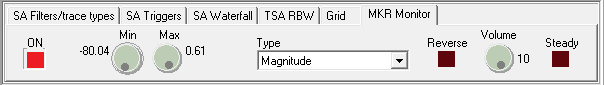
You can define the amplitude range with the Min and Max knobs. The amplitude range is -80 dBm to 0 dBm in the above example.

With the Type set to Magnitude, you will get an audible tone that will vary from 100Hz to 10kHz on a linear scale over the range -80dBm to 0dBm.

E.g., an about 5 kHz tone will be out if the selected marker indicates a -40 dBm signal. The volume of the audio tone will also follow the amplitude of the signal indicated by the marker in percent. So in the example above, the volume of the 5 kHz tone will be half the overall volume set with the Volume knob.

You can activate a flat volume with the Steady button if you do not want it to follow the amplitude of the marker.

The Reverse button reverses the tone scale. You will get a 10kHz tone with the -80dBm marker and a 100Hz tone with the 0dBm.

The types Frequency and Frequency to/from center configure the monitor to produce a tone related to the frequency locked by the marker rather than the amplitude. The Bandwidth field of the selected marker determines the frequency range of the above two types. These two types are allowed only in Spectrum Analyzer mode. A magnitude type is a default in SNA or VNA operations. Here is an example of using the Frequency types with the Spectrum Analyzer:

Create a new marker from the Edit SA markers table window:

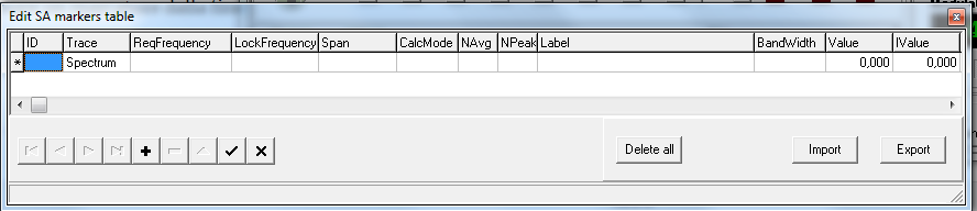
Fill in the ReqFrequency field with 145000000 and Bandwidth with 100000, for example.

The LockFrequency field is filled at the spectrum analyzer start. The LockFrequency field will be the strongest signal frequency inside the range of the Bandwidth field.

When the Marker Monitor is set to type Frequency, SATSAGEN generates a 100Hz of audible tone when the above marker has a LockFrequency field of 144,950 MHz. While a 10kHz tone will be generated at 145,050 kHz.

With the marker monitor activated of type Frequency to/from center, a 100 Hz tone will be generated if the detected signal is exactly at the required frequency of the marker, in the example 145 MHz, while 10 kHz tones will be generated if the signal found at 144.950 MHz or 145.050 MHz.

The Reverse function reverses the tone scale in both of the above types.

Waterfall

The new Waterfall of this version provides a fixed resolution configurable in Settings->Appearance instead of a dynamic resolution of the previous Waterfall. This means that any resizing of the window does not cause the waterfall to be reset.

From this version, it is possible to activate the Waterfall on an independent window rather than having it integrated into the main application window.

In the control panel of the new integrated Waterfall, there are the new Stand-alone, Max PeakH and Res Adapt controls:

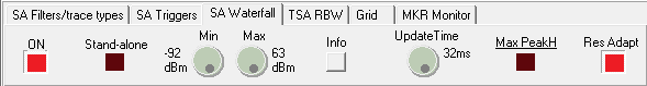
The Stand-Alone control starts the Waterfall on an independent Window.

The Max PeakH function allows the data acquired between one UpdateTime and another not to be lost. For example, if UpdateTime is set to 500ms and Max PeakH is off, every half second a line will be added to the waterfall with the spectrum of the instant, while with Max PeakH on each line will be the max hold of the last 500ms. By clicking on the label Max PeakH, it is possible to select an Average update process rather than a max hold.

The Res Adapt function adapts the data resolution to the pixel dimension of the waterfall window so that any signals present “narrower” than the video resolution is anyway displayed. If you use the zoom function, the Res Adapt function should be turned off to take advantage of the maximum detail available.

The functions just seen are also present on the Waterfall panel on an independent window:

Furthermore, the Vertical controls are available on this panel for orienting the Waterfall vertically, Levels for displaying the legend with the colors assigned for each signal amplitude, a Time Axis for displaying the abscissa with time information, Time Labels for a display of time labels inside the Waterfall, Hold to stop the display and finally ZReset to reset the zoom to the initial values.

Auto-export spectrum analyzer data

From this version, it is possible to set the automatic export of spectrum data in comma-delimited text format. There are all settings for this function In Settings->Logs/Export:

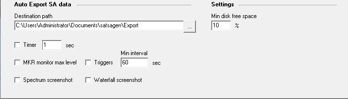
First of all, it is necessary to define a destination path for the text files that SATSAGEN will create before enabling the automatic export. Sets the desired path in the Destination path field and Min disk free space with the free disk threshold value.

Once the destination path and the minimum free disk threshold have been defined, the enabling takes place with the choice of the method with which the triggering of the automatic export will take place.

By enabling the Timer control, the export will take place at every interval in seconds specified in the adjacent field.

By selecting the MKR monitor max level, the export will be triggered when a signal monitored by the MKR monitor function (previously seen in the Marker monitor paragraph) reaches the level defined by the Max knob on the MKR monitor panel.

If the Triggers checkbox is selected, the export will take place as a result of the activation of one of the triggers set up in the SA Triggers panel.

Both the above MKR monitor max level and Trigger methods are conditioned by a minimum reactivation interval defined by the Min interval field, within which any triggers will be ignored.

The above methods are not exclusive, so any combination of Timer configuration, Triggers, and MKR monitor max level is allowed.

Finally, if the Spectrum screenshot and/or Waterfall screenshot controls are activated, the relative screenshots will also be taken with each automatic export that will be activated.

Save/load SNA calibration data

From this version, there is a function that allows the saving and loading of the SNA calibration data from a file.

This function is accessed via the menu items under File->Calibration data:

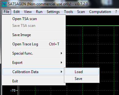
If you are using the VNA, the above menu items will act like the Load and Save buttons of the VNA Calibration panel.

Restore window size and position

By enabling the Restore saved window size and positions function from Settings->Appearance, the dimensions and position of the main window, of the integrated waterfall, and the independent window will be saved when the application is closed and re-applied when it is restarted.

The maximized or minimized states of the main window will also be saved and restored when the application is restarted.

Gesture

By activating the Gesture enabled control from Settings->Appearance, the following gestures are available within the scope window of the spectrum Analyzer, provided that the mouse cursor is within the Scope of the Spectrum Analyzer but away from the edges and from any cursors present:

  • Central frequency. The central frequency will vary with the defined steps by holding down the left mouse button and moving horizontally. Imagine viewing the spectrum as a sheet of paper: shifting to the left will increase the center frequency, and shifting to the right will decrease it.
  • Span. By holding down the right button (or the middle mouse button) and moving horizontally, the span will increase in the left direction and decrease in the right direction.
  • Zoom. Holding down any of the mouse buttons and simultaneously holding down the Ctrl key, vertical and horizontal mouse movement will respectively vertically and horizontally zoom the displayed spectrum. On touch screens, the horizontal zoom will be managed using the classic two-finger gesture on the screen.

The above gestures will work reversed If the Gesture reversed checkbox is enabled from Settings->Appearance. E.g., the central frequency will increase if you hold down the left mouse button and move it to the right.

Spectrum analyzer resource monitor

An automatic PC processing time control feature is enabled by default when the SATSAGEN spectrum analyzer is running. This function detects any exceeding of pre-set timeout thresholds, in particular on the acquisition and processing times of data from the SDR devices, and intervenes by progressively reducing the workload to bring the times back below the above thresholds to avoid slowdowns or hangs of the user interface. For example, this function can intervene by reducing the FFT size or turning off the Fast cycle when it detects that these settings can lead to slowdowns or blockages of the application. Automatic interventions are signaled with the opening of the trace log window and an explanatory message of the intervention.

It is possible to disable or re-enable this feature via the Settings->SA resource monitor menu.